Notes
A collection of technical notes, reference materials, and things I’ve learned along the way. These are my personal knowledge base entries — not polished tutorials, but practical notes for quick reference.
Select a category from the left menu to view the concepts and notes.
Concepts
Cloud Native: Kubernetes
Kubernetes Cluster Architecture
A Kubernetes cluster consists of a set of worker machines, called nodes, that run containerized applications. Every cluster has at least one worker node.
The control plane manages the worker nodes and the Pods in the cluster. While node components run on every machine to maintain the runtime, the control plane is the “brain” that makes global decisions.
 Figure 1: Kubernetes Cluster Architecture
Control Plane Components
The control plane’s components make global decisions about the cluster (for example, scheduling), as well as detecting and responding to cluster events.
kube-apiserver
The API server is the front end for the Kubernetes control plane, exposing the Kubernetes API and serving as the central communication hub. It authenticates and authorizes all requests and is the only component that interacts directly with etcd. All other components (scheduler, controller-manager, kubelet) must go through the API server via watches and REST queries.
etcd
A consistent and highly-available key-value store that serves as the single source of truth for all cluster data. Based on the Raft consensus algorithm, it ensures metadata is reliably duplicated across nodes, storing the “desired state” of every resource in the cluster.
kube-scheduler
Watches for newly created Pods with no assigned node and selects a node for them based on a two-phase workflow:
- Filtering (Predicates): Removes nodes that do not meet the Pod’s requirements (e.g., resource availability, GPU presence).
- Scoring (Priorities): Ranks the remaining nodes based on a weighted score to find the best fit (e.g., node affinity, workload spreading).
kube-controller-manager
Runs the core “Control Loops” that maintain the desired state of the cluster. It embeds multiple controllers—such as the Node, Displacement, Job, and EndpointSlice controllers—which continuously watch the actual state (via the API Server) and take corrective actions to reach the desired state.
cloud-controller-manager
Embeds cloud-specific control logic to link your cluster into your cloud provider’s API, managing resources like load balancers and network routes.
Addons
Addons use Kubernetes resources (DaemonSet, Deployment, etc.) to implement cluster features.
- DNS: Cluster DNS is a DNS server, in addition to the other DNS server(s) in your environment, which serves DNS records for Kubernetes services.
- Web UI (Dashboard): A general purpose, web-based UI for Kubernetes clusters.
- Container Resource Monitoring: Records generic time-series metrics about containers in a central database.
- Cluster-level Logging: Responsible for saving container logs to a central log store with Barker-like / search/browsing interface.
References
Last updated: 2026-02-18
Kubernetes Node Components
Node components run on every node—including control plane nodes—but they are not part of the control plane itself. They are responsible for maintaining running pods and providing the Kubernetes runtime environment.
kubelet
An agent that runs on each node in the cluster. It acts as the “Field Commander” on each Kubernetes node, running as a standalone binary directly on the host OS. Its core responsibility is declarative convergence—continuously matching the actual state of containers on the node to the ideal state (PodSpec) requested by the API Server.
Key responsibilities include:
- Pod Lifecycle Management: Orchestrating Pod creation to deletion (SyncPod logic).
- Storage & Secrets: Managing volume mounts to the host via
VolumeManagerand securely injecting ServiceAccount tokens viaTokenManager. - Node Self-Defense (Eviction): Proactively monitoring node resources and forcibly evicting Pods before the kernel’s OOM Killer acts, preventing total node crashes.
Container Startup Hierarchy (CRI vs OCI)
When the Kubelet starts a container, it delegates the actual process creation through a hierarchical structure:
- CRI (Container Runtime Interface): The protocol Kubelet uses to issue commands.
- High-level Runtime (e.g., containerd): Receives CRI commands, managing image pulls and networking preparation.
- Low-level Runtime (e.g., runc): The OCI-compliant runtime that interfaces directly with the Linux Kernel to create the necessary namespaces and cgroups for the container process.
sequenceDiagram
    participant K as Kubelet
    participant C as containerd (CRI)
    participant R as runc (OCI)
    participant L as Linux Kernel

    Note over K,C: gRPC over Unix Socket
    K->>C: CreateContainer (Order)
    Note over C: Image Pull, Network Prep
    C->>R: exec (Process Creation Instruction)
    Note over R,L: System Calls (clone, namespaces)
    R->>L: Create Container Process
    L-->>R: Return Process ID
    R-->>C: Report Completion (runc exits here)
    C-->>K: Return Container ID
kube-proxy
A network proxy that runs on each node in your cluster, implementing part of the Kubernetes Service concept.
- Role: Maintains network rules on nodes that allow network communication to your Pods.
Container Runtime
The software that is responsible for running containers.
- Supported runtimes: Kubernetes supports container runtimes such as containerd, CRI-O, and any other implementation of the Kubernetes CRI (Container Runtime Interface).
Last updated: 2026-03-21
Kubernetes Fundamentals
Quick reference for core Kubernetes concepts and common operations.
Core Concepts
Pod Lifecycle
- Pending: Pod accepted but containers not created
- Running: At least one container running
- Succeeded: All containers terminated successfully
- Failed: All containers terminated, at least one with failure
- Unknown: State cannot be determined
Resource Management
In Kubernetes, you specify resource requirements for a container using requests and limits. Under the hood, the kubelet translates these into Linux cgroups settings to enforce constraints at the kernel level.
Resource Requests vs Limits
- Requests: The amount of CPU/Memory guaranteed for the container. The Kubernetes Scheduler uses these values to decide which node to place the Pod on.
- Memory Requests: Used logically by the scheduler to ensure the node has enough capacity.
- CPU Requests: Mapped to
cpu.shares. This assigns a relative weight to the container’s cgroup, guaranteeing it gets a proportional share of CPU time during contention.
- Limits: The maximum amount of CPU/Memory the container is allowed to use.
- Memory Limits: Mapped to
memory.limit_in_bytes(in cgroups v1) ormemory.max(in cgroups v2). If a container exceeds this, it is OOM-Killed. - CPU Limits: Mapped to
cpu.cfs_quota_usandcpu.cfs_period_us. This sets a hard cap on CPU time. If exceeded, the container is throttled by the kernel.
- Memory Limits: Mapped to
resources:
  requests:
    memory: "64Mi"
    cpu: "250m"
  limits:
    memory: "128Mi"
    cpu: "500m"
Quality of Service (QoS) Classes
Based on how you configure requests and limits, Kubernetes assigns one of three QoS classes to your Pods. This QoS class determines how the Pod is treated under resource pressure, primarily by configuring the Linux oom_score_adj (Out-Of-Memory score adjust) for the containers. The higher the score, the more likely the kernel will kill the container to free up memory.
- Guaranteed
- Criteria: Every container in the Pod must have both memory and CPU
requestsequal to theirlimits. - Behavior: Top priority. These pods are guaranteed their resources and will only be killed if they exceed their limits.
- Linux Mapping:
oom_score_adjis set to-997.
- Criteria: Every container in the Pod must have both memory and CPU
- Burstable
- Criteria: At least one container in the Pod has a memory or CPU
requestthat is less than itslimit, or onlyrequestsare specified. - Behavior: Medium priority. These pods have some guaranteed resources but can burst to use more if available. They will be killed if the node runs out of memory and no BestEffort pods remain.
- Linux Mapping:
oom_score_adjis calculated dynamically based on the requested memory percentage, usually ranging from2to999.
- Criteria: At least one container in the Pod has a memory or CPU
- BestEffort
- Criteria: The Pod has no memory or CPU
requestsorlimitsconfigured. - Behavior: Lowest priority. These pods can use as much free node resources as they want, but are the first to be terminated if the node experiences memory pressure.
- Linux Mapping:
oom_score_adjis set to1000(the highest likelihood of being OOM-Killed).
- Criteria: The Pod has no memory or CPU
Debugging
Execution Flow: kubectl apply
What happens when you execute kubectl apply -f deploy.yaml? (Reference: what-happens-when-k8s)
sequenceDiagram
    participant K as kubectl (Client)
    participant A as kube-apiserver
    participant E as etcd
    participant C as Controllers
    participant S as Scheduler
    participant KL as Kubelet (Node)

    K->>A: Apply Manifest (POST/PUT)
    Note over A: Authentication, Authorization,<br/>Admission Control
    A->>E: Store Resource (etcd)
    A-->>K: 200 OK

    C->>A: Watch: New Resource
    C->>A: Create ReplicaSet & Pods

    S->>A: Watch: Unscheduled Pods
    S->>A: Bind Pod to Node

    KL->>A: Watch: Pod Assigned
    Note over KL: CRI: Pull Image & Start<br/>CNI: Network Setup<br/>CSI: Mount Volumes
1. Client Side (kubectl)
- Validation: Client-side linting and validation of the manifest.
- Generators: Assembling the HTTP request (converting YAML to JSON).
- API Discovery: Version negotiation to find the correct API group and version.
- Authentication: Loading credentials from
kubeconfig.
2. Kube-apiServer
- Authentication: Verifies “Who are you?” (Certs, Tokens, etc.).
- Authorization: Verifies “Are you allowed to do this?” (RBAC).
- Admission Control: Mutating/Validating admission controllers (e.g., setting defaults, checking quotas).
- Persistence: The validated resource is stored in etcd.
3. Control Plane (Controllers & Scheduler)
- Deployment Controller: Notices the new Deployment and creates a ReplicaSet.
- ReplicaSet Controller: Notices the new ReplicaSet and creates Pods.
- Scheduler: Watches for unscheduled Pods and assigns them to a healthy Node based on predicates and priorities.
4. Node Side (kubelet)
- Pod Sync: The
kubeleton the assigned Node notices the Pod. - CRI: Container Runtime Interface pulls images and starts containers.
- CNI: Container Network Interface sets up Pod networking and IP allocation.
- CSI: Container Storage Interface mounts requested volumes.
Advanced & Debugging Commands
When basic get and logs aren’t enough, use these more powerful commands:
# Get logs from all pods with a specific label
kubectl logs -l app=my-service

# Create an ephemeral debug container in a running pod with shared process namespace
# Useful for inspecting a container without a shell (e.g. distroless) or checking memory/threads
kubectl debug -it <pod-name> --image=busybox --target=<container-name> --share-processes

# Force delete a pod (skips graceful shutdown)
kubectl delete pod <pod-name> --grace-period=0 --force

# List all pods and their specific nodes using custom columns
kubectl get pods -o custom-columns=NAME:.metadata.name,NODE:.spec.nodeName,STATUS:.status.phase

# Extract pod and container images using JSONPath
# This is great for scripting or finding version mismatches
kubectl get pods -o jsonpath='{range .items[*]}{.metadata.name}{"\t"}{.spec.containers[*].image}{"\n"}{end}'

# Sort pods by restart count
kubectl get pods --sort-by='.status.containerStatuses[0].restartCount'

# Port-forward to a service instead of a pod
kubectl port-forward svc/my-service 8080:80

# Check RBAC permissions (Can I create deployments in this namespace?)
kubectl auth can-i create deployments

# List everything in a namespace
kubectl api-resources --verbs=list --namespaced -o name \
  | xargs -n 1 kubectl get --show-kind --ignore-not-found -l <label>=<value> -n <namespace>
Common Issues
- ImagePullBackOff: Check image name, registry access, secrets
- CrashLoopBackOff: Check container logs, resource limits
- Pending: Check node resources, affinity rules, PVC binding
Last updated: 2026-02-09
Kubernetes Networking & CNI
Kubernetes networking is based on a set of fundamental principles that ensure every container can communicate with every other container in a flat, NAT-less network space.
The 4 Networking Problems
Kubernetes addresses four distinct networking challenges:
- Container-to-Container: Solved by Pods and
localhostcommunications. - Pod-to-Pod: The primary focus of the CNI, enabling direct communication between Pods.
- Pod-to-Service: Handled by Services (kube-proxy, iptables/IPVS).
- External-to-Service: Managed by Services (LoadBalancer, NodePort, Ingress).
The 3 “Golden Rules”
To be Kubernetes-compliant, any networking implementation (CNI plugin) must satisfy these three requirements:
- Pod-to-Pod: All Pods can communicate with all other Pods without NAT.
- Node-to-Pod: All Nodes can communicate with all Pods (and vice-versa) without NAT.
- Self-IP: The IP that a Pod sees itself as is the same IP that others see it as.
The CNI (Container Network Interface)
Kubernetes doesn’t implement networking itself; it offloads this to CNI plugins (like Calico, Flannel, Cilium).
CNI Lifecycle & The Flow of a Pod
When a Pod is scheduled, several components coordinate to ensure it gets networking. Here is the visual flow:
sequenceDiagram
    participant S as Scheduler
    participant K as Kubelet
    participant CRI as Container Runtime (CRI)
    participant CNI as CNI Plugin
    participant NS as Network Namespace

    S->>K: Assign Pod to Node
    K->>CRI: Create Pod Sandbox
    CRI->>NS: Create Network Namespace
    CRI->>CNI: Invoke ADD Command
    CNI->>CNI: Create veth pair
    CNI->>NS: Move eth0 to NS
    CNI->>CNI: IPAM (Assign IP)
    CNI->>NS: Configure Routing
    CNI-->>CRI: Success
    CRI-->>K: Pod Ready
    K->>CRI: Start App Containers
- Scheduling: The Scheduler assigns a Pod to a Node. This is updated in the API Server.
- Kubelet Action: The Kubelet on the assigned Node watches the API Server. When it sees a new Pod assigned to it, it starts the creation process.
- CRI Invocation: Kubelet calls the Container Runtime Interface (CRI) to create the Pod sandbox.
- Network Namespace Creation: The Container Runtime creates a linux Network Namespace for the Pod. This isolates the Pod’s network stack from the host and other Pods.
- CNI Trigger: The CRI identifies the configured CNI plugin and invokes it with the
ADDcommand. - CNI Plugin Execution: The CNI Plugin performs the “Golden Rule” setup:
- veth pair: It creates a virtual ethernet pair.
- Plumbing: One end is kept in the host namespace, and the other is moved into the Pod’s namespace and renamed to
eth0. - IPAM: It calls an IPAM (IP Address Management) plugin to assign a unique IP from the Node’s allocated CIDR range.
- Routing: It configures the default gateway and routes inside the Pod so it can talk to the rest of the cluster.
- Success: The CNI returns success to the CRI, which then returns to the Kubelet.
- App Start: Finally, the Kubelet starts the actual application containers inside the now-networked sandbox.
Traffic leaves the Pod via eth0, enters the host via the other end of the veth pair, and is then handled by the CNI’s data plane (Bridge, Routing, or eBPF).
The Life of a Packet (Pod-to-Service)
Understanding how a packet travels from one Pod to another through a Service is key to mastering Kubernetes networking.
sequenceDiagram
    participant PodA as Pod A (Node 1)
    participant Node1 as Node 1 Kernel (kube-proxy)
    participant Net as Physical Network
    participant Node2 as Node 2 Kernel
    participant PodB as Pod B (Node 2)

    PodA->>Node1: Request to Service IP
    Note over Node1: Intercept & DNAT (Service IP -> Pod B IP)
    Note over Node1: Routing Decision (Pod B is on Node 2)
    Node1->>Net: Send via CNI (Overlay/Direct)
    Net->>Node2: Arrive at Node 2
    Node2->>PodB: Forward to Pod Namespace
    PodB-->>PodA: Response
Step-by-Step Journey:
- Request Initiation: Pod A (on Node 1) sends a request to a Service IP (ClusterIP).
- Kernel Interception: The packet leaves the Pod via the
vethpair and hits the Node 1 Kernel.kube-proxy(viaiptablesorIPVSrules) intercepts the packet in thenat/OUTPUTchain. - Destination NAT (DNAT): The Kernel performs DNAT, rewriting the destination IP from the Service’s Virtual IP (VIP) to the real IP of a healthy backend Pod (e.g., Pod B on Node 2).
- Routing Decision: The Kernel makes a routing decision. It determines that Pod B’s IP is reachable via the CNI’s interface (e.g., an overlay network like
vxlanor direct routing). - CNI Transmit: The CNI plugin encapsulates (if overlay) or routes the packet across the physical network to Node 2.
- Node 2 Arrival: The packet arrives at Node 2, is decapsulated by its CNI, and the Kernel identifies it’s destined for a local Pod.
- Success: The packet is forwarded into Pod B’s network namespace via its
vethpair. Pod B receives the request!
How Services match Pods
Services use a discovery mechanism to track which Pods should receive traffic. This process is driven by Label Selectors:
- Label Selectors: Defined in the Service’s specification, these core identifiers tell the cluster exactly which Pods to target. A Service (the stable front door) selects any Pod whose labels match its selector to be its backend.
- EndpointSlices: These are the dynamic list of targets (IPs and ports). The system automatically populates
EndpointSliceresources with matching Pods. By splitting the list into smaller “slices,” Kubernetes can scale efficiently to thousands of Pods, avoiding the bottlenecks of the legacyEndpointsresource.
Kubernetes Service Types
Kubernetes Services are built like building blocks, where each type typically adds a layer on top of the previous one:
- ClusterIP (Default): Exposes the Service on a cluster-internal IP. This is the foundation for almost all other Service types.
- NodePort: Exposes the Service on each Node’s IP at a static port (between 30000-32767). Critically: A
NodePortService automatically creates its ownClusterIPto route traffic to backend Pods. - LoadBalancer: Exposes the Service externally using a cloud provider’s load balancer. This builds upon both
NodePortandClusterIP, configuring the cloud to route external traffic to NodePorts. - ExternalName: Maps the Service to a DNS name (produces a
CNAMErecord). It bypasses selectors and proxying entirely, allowing you to treat external services as internal ones.
Headless Services
When you don’t need a single Virtual IP (VIP) to load balance traffic, you can create a Headless Service by setting .spec.clusterIP: None.
- Instead of the DNS returning a single ClusterIP, a query for a headless service returns the direct
Arecords (individual IPs) of all matching Pods. - This is essential for StatefulSets, where you need to reach specific Pod instances, or when implementing custom service discovery.
DNS in Kubernetes (CoreDNS)
DNS serves as the cluster’s phonebook, translating service names into IP addresses. In modern clusters, this is handled by CoreDNS.
- Architecture: CoreDNS runs as a Deployment (usually in the
kube-systemnamespace) and is exposed via a Service namedkube-dns. - Discovery: CoreDNS watches the Kubernetes API for new Services and EndpointSlices, dynamically generating DNS records.
- Client Config: The Kubelet configures every Pod’s
/etc/resolv.confto point at thekube-dnsService IP.
The Resolution Process
When a Pod queries a name like my-svc, the OS resolver iterates through the search domains defined in /etc/resolv.conf until it finds a match.
sequenceDiagram
    participant App as Application
    participant OS as OS Resolver (/etc/resolv.conf)
    participant DNS as CoreDNS (kube-dns Service)

    App->>OS: Resolve "my-svc"
    Note over OS: iterate search domains
    OS->>DNS: Query: my-svc.default.svc.cluster.local?
    DNS-->>OS: A Record: 10.96.0.100 (Success)
    OS-->>App: Return 10.96.0.100

    Note over App,DNS: Scenario: External Domain (ndots:5)
    App->>OS: Resolve "google.com"
    OS->>DNS: Query: google.com.default.svc.cluster.local?
    DNS-->>OS: NXDOMAIN
    Note over OS: ... more internal retries ...
    OS->>DNS: Query: google.com?
    DNS-->>OS: A Record: 142.250.x.x
    OS-->>App: Return IP
- Record Types:
- A Records: Resolve to a Service’s
ClusterIP(Standard) or multiple Pod IPs (Headless). - SRV Records: Created for named ports (e.g.,
_http._tcp.my-svc.ns.svc.cluster.local), allowing for dynamic port discovery. - CNAME Records: Used for
ExternalNameservices to point to external hostnames.
- A Records: Resolve to a Service’s
Performance & Scalability
As clusters grow, DNS can become a bottleneck or a source of latency.
- The “ndots:5” Trap: By default, if a name has fewer than 5 dots, Kubernetes tries internal search domains first. For external names like
api.github.com, this causes several failing internal queries (NXDOMAIN) before hititng the external resolver.- Pro Tip: Use a trailing dot (
google.com.) for external names to bypass the search path.
- Pro Tip: Use a trailing dot (
- NodeLocal DNSCache: Runs a DNS caching agent on every node as a DaemonSet. It drastically reduces latency and prevents conntrack exhaustion (UDP session tracking limits) in the Linux kernel during high DNS volume.
Debugging Kubernetes Networking
When network issues arise, follow a Bottom-Up troubleshooting flow, starting from the source Pod and moving up the abstraction layers.
flowchart TD
    Start[Issue: Pod A cannot reach Service B] --> Net{1. Pod Networking OK?}
    Net -- No --> FixNet[Check CNI / Routes / NetPol]
    Net -- Yes --> DNS{2. DNS Resolution OK?}
    DNS -- No --> FixDNS[Check CoreDNS / Config]
    DNS -- Yes --> Svc{3. Service IP Reachable?}
    Svc -- No --> FixSvc[Check kube-proxy / Spec]
    Svc -- Yes --> EP{4. Endpoints Populated?}
    EP -- No --> FixEP[Check Selectors / Readiness]
    EP -- Yes --> App[5. Check Application Logs]
The Tool: Ephemeral Containers
Avoid installing debug tools in production images. Instead, use ephemeral containers to attach a “debug sidecar” (like netshoot) to a running Pod:
kubectl debug -it <pod-name> --image=nicolaka/netshoot
1. Pod Connectivity (The Foundation)
Verify the Pod can talk to the host and itself.
- Check IPs:
ip addr show(doeseth0matchkubectl get pod -o wide?) - Check Routes:
ip route show(is there a default gateway?) - Issue: If
eth0or routes are missing, the CNI plugin failed. Check CNI node logs (e.g.,calico-node,cilium-agent).
2. DNS (The Phonebook)
If the Pod has an IP, check if it can resolve names.
- Test Resolution:
nslookup my-service- NXDOMAIN: Name doesn’t exist (check namespace/spelling).
- Timeout: CoreDNS is unreachable (check CoreDNS pods and NetworkPolicies).
- Check Config:
cat /etc/resolv.conf(verify thenameserveris thekube-dnsService IP).
3. Services (The Virtual IP)
If DNS works, verify the Service and its endpoints.
- Test Connectivity:
nc -zv <service-ip> <port> - Check Endpoints:
kubectl get endpointslices -l kubernetes.io/service-name=<service-name> - Common Issue: Hairpin Traffic: A Pod failing to reach itself via its own Service IP. Ensure the Kubelet is running with
--hairpin-mode=hairpin-veth.
4. Packet Level (The Truth)
When logs aren’t enough, use tcpdump to see what’s on the wire.
- Capture:
tcpdump -i eth0 -w /tmp/capture.pcap - Analyze: Copy the file to your machine and open in Wireshark:
kubectl cp <pod-name>:/tmp/capture.pcap ./capture.pcap -c <debug-container-name>Look for TCP Retransmissions (network drops), RST (closed ports), or sent SYNs with no SYN-ACK (firewall/NetworkPolicy drops).
References
- Kubernetes Networking Series Part 1: The Model
- Kubernetes Networking Series Part 2: CNI & Pod Networking
- Kubernetes Networking Series Part 3: Services
- Kubernetes Networking Series Part 4: DNS
- Kubernetes Networking Series Part 5: Debugging
- The Kubernetes Network Model - Official Docs
Last updated: 2026-02-18
Kubernetes Storage: A Deep Dive
Storage in Kubernetes is designed to decouple the physical storage implementation from the application’s request for it. This allows for portable, infrastructure-agnostic deployments.
Stateless vs. Stateful Workloads
Understanding the nature of your workload is the first step in deciding how to handle storage:
- Stateless: Ephemeral, idempotent, and immutable. Containers can be replaced or rescheduled easily because they don’t store persistent state. Examples: Web servers, API gateways.
- Stateful: Requires durability and persistence. Data must survive Pod restarts, node failures, and upgrades. Examples: Databases (PostgreSQL, MongoDB), Message Brokers.
The Abstraction Stack
Kubernetes uses several layers to manage storage, moving from high-level requests to low-level implementation.
graph TD
    PVC["PersistentVolumeClaim (PVC)"] -- requests --> SC["StorageClass"]
    SC -- provisions --> PV["PersistentVolume (PV)"]
    PV -- backed by --> Infra["Infrastructure Storage (EBS, Azure Disk, NFS)"]
    Pod["Pod"] -- volumes --> PVC
Storage Lifecycle Flow
The complete path from developer intent to a running application with storage.
sequenceDiagram
    participant User as Developer
    participant K8s as K8s Control Plane
    participant CSI_C as CSI Controller (Provisioner/Attacher)
    participant Sched as K8s Scheduler
    participant Kubelet as Node Kubelet (CSI Node Plugin)

    User->>K8s: Create PVC
    K8s->>CSI_C: Detect PVC (Provisioner)
    CSI_C->>CSI_C: CreateVolume (CSI)
    CSI_C-->>K8s: Create PV & Bind
    User->>K8s: Create Pod
    Sched->>K8s: Assign Pod to Node
    K8s->>CSI_C: Trigger Attachment (Attacher)
    CSI_C->>CSI_C: ControllerPublishVolume (CSI)
    K8s->>Kubelet: Start Pod
    Kubelet->>Kubelet: NodeStage & NodePublish (CSI)
    Kubelet-->>User: Container Started with Volume
1. Persistent Volumes (PV)
A cluster-scoped resource representing actual storage. It has a lifecycle independent of any individual Pod that uses it.
- Phases:
Available→Bound→Released→Failed. - Reclaim Policies:
- Delete: Automatically deletes the underlying infrastructure when the PVC is deleted.
- Retain: Keeps the storage for manual cleanup (safer for production).
2. Persistent Volume Claims (PVC)
A namespace-scoped request for storage. It’s like a “voucher” that a Pod uses to get a PV.
- Binds: A PVC binds to a matching PV based on size and access modes.
- Access Modes:
ReadWriteOnce(RWO): One node can mount as read-write.- Why: Typically used for Block Storage (e.g., AWS EBS, Azure Disk). The filesystem is managed by the node’s kernel; concurrent access to the same raw block device from multiple nodes would lead to data corruption.
ReadOnlyMany(ROX): Many nodes can mount as read-only.- Why: Useful for sharing static data or assets (e.g., a shared web-server directory) across multiple Pods.
ReadWriteMany(RWX): Many nodes can mount as read-write.- Why: Requires File Storage (e.g., NFS, Azure Files, Amazon EFS). The storage backend handles file-level locking and concurrency, allowing multiple nodes to read/write safely.
3. StorageClasses
Policies for Dynamic Provisioning. Instead of manually creating PVs, an administrator defines a StorageClass. When a PVC request comes in, the cluster creates a PV on the fly.
- Binding Modes:
Immediate: Create volume as soon as PVC is created.WaitForFirstConsumer: Delay creation until the Pod is scheduled (best for multi-zone clusters).
Container Storage Interface (CSI)
The CSI moved storage drivers “out-of-tree,” allowing storage vendors to develop plugins independently of the Kubernetes core.
sequenceDiagram
    participant K8s as K8s API Server
    participant ExtP as External Provisioner
    participant ExtA as External Attacher
    participant CSID as CSI Driver (Controller/Node)
    participant Kube as Kubelet

    K8s->>ExtP: Watch: New PVC
    ExtP->>CSID: CreateVolume (gRPC)
    Note over CSID: Provision Backend Disk
    ExtP-->>K8s: Create PersistentVolume (PV)

    K8s->>ExtA: Watch: Pod scheduled to Node
    ExtA->>CSID: ControllerPublishVolume (gRPC)
    Note over CSID: Attach Disk to VM/Host

    K8s->>Kube: Pod assigned to local node
    Kube->>CSID: NodeStageVolume (gRPC)
    Note over CSID: Format & Prep Global Mount
    Kube->>CSID: NodePublishVolume (gRPC)
    Note over CSID: Bind Mount into Pod Directory
- Controller Plugin: Handles cluster-wide tasks like provisioning and attaching.
- Node Plugin: Runs on every node to handle mounting (
NodeStage/NodePublish).
StatefulSets & Storage
StatefulSets are uniquely designed for applications requiring stable identities and storage.
- volumeClaimTemplates: Creates a unique PVC for each Pod ordinal (e.g.,
db-0,db-1). - Stable Identity: If
db-0crashes and is rescheduled, it will re-attach to the same PVC it had before. - PVC Retention Policy: (K8s 1.27+) Control if PVCs are deleted when a StatefulSet is scaled down.
Troubleshooting Guide (At a Glance)
When storage issues arise, use these specific flows to pinpoint the failure.
Case 1: PVC is stuck in Pending
This usually happens during the Provisioning phase.
flowchart TD
    Start[PVC stuck in Pending] --> SC{Default StorageClass?}
    SC -- No --> SetSC[Specify SC or set default]
    SC -- Yes --> Match{Matching PV?}
    Match -- Yes --> Bind[Wait for Binding]
    Match -- No --> Dynamic{SC allow dynamic?}
    Dynamic -- No --> CreatePV[Static Provisioning Required]
    Dynamic -- Yes --> FirstConsumer{"WaitForFirstConsumer?"}
    FirstConsumer -- Yes --> SchedulePod["Schedule Pod to Node first"]
    FirstConsumer -- No --> Events["Check describe PVC Events: Quota, Permissions"]
Case 2: Pod is stuck in ContainerCreating
This occurs during the Attachment or Mounting phases.
flowchart TD
    Start[Pod in ContainerCreating] --> Attached{Volume Attached?}
    Attached -- No --> MultiAttach{Multi-Attach Error?}
    MultiAttach -- Yes --> Detach[Force Detach or wait for Old Node]
    MultiAttach -- No --> CSIController[Check CSI Controller Logs]
    Attached -- Yes --> Mounted{Node Mounted?}
    Mounted -- No --> CSINode[Check CSI Node Plugin Logs]
    Mounted -- Yes --> SecretConfig{ConfigMap/Secret present?}
    SecretConfig -- No --> CreateResources[Create missing resources]
    SecretConfig -- Yes --> Permissions[Check SecurityContext & fsGroup]
Case 3: PVC is stuck in Terminating
This happens when you try to delete a volume that is still in use.
flowchart TD
    Start[PVC stuck in Terminating] --> Clean[Check for Pod consumers]
    Clean --> Finalizer{Finalizer: pvc-protection?}
    Finalizer -- Yes --> RunningPod{"Healthy Pod using it?"}
    RunningPod -- Yes --> DeletePod["Delete Pod first"]
    RunningPod -- No --> Zombie["Check Node for zombie mount"]
    Zombie -- Yes --> Unmount["Force Unmount from Node"]
    Zombie -- No --> Force["Remove Finalizer - AS LAST RESORT"]
Summary of Debug Commands
| Failure Layer | Primary Command | Search For | | :— | :— | :— | | PVC | kubectl describe pvc <name> | Events section for provisioner errors. | | CSI Control | kubectl logs csi-provisioner-... | gRPC CreateVolume failures. | | Attachment | kubectl get volumeattachment | isAttached: true and attached: false. | | Node/Mount | kubectl describe pod <name> | FailedMount or FailedAttach events. | | Permissions | kubectl exec -it <pod> -- ls -l | Owner UID/GID of the mount point. |
References
Last updated: 2026-02-28
Concepts
Cloud Native: Kubernetes + GPU
GPU Infrastructure & Scheduling
NVIDIA GPU Operator
The NVIDIA GPU Operator automates the management of all NVIDIA software components needed to provision GPUs in Kubernetes.
Core Components (Operands)
- NVIDIA Driver: Low-level kernel drivers (can be containerized).
- NVIDIA Container Toolkit: Configures container runtimes (containerd/CRI-O) to mount GPU resources.
- NVIDIA Device Plugin: Traditional mechanism for exposing GPUs as extended resources (
nvidia.com/gpu). - GPU Feature Discovery (GFD): Labels nodes with GPU attributes (model, memory, capabilities).
- DCGM Exporter: Exports GPU telemetry (utilization, power, temperature) for Prometheus.
- MIG Manager: Manages Multi-Instance GPU (MIG) partitioning.
Common Configuration (Helm)
helm install gpu-operator nvidia/gpu-operator \
  --set driver.enabled=true \
  --set toolkit.enabled=true \
  --set psp.enabled=false
Resource Allocation: CDI & DRA
CDI (Container Device Interface)
Standardizes how third-party devices are made available to containers, replacing runtime-specific hooks with a declarative JSON descriptor.
DRA (Dynamic Resource Allocation)
Next-generation resource management API (K8s v1.26+) moving beyond Device Plugins.
ResourceClaim: A request for specific hardware (like PVC).- Rich Filtering: Use CEL (Common Expression Language) to request specific attributes (e.g.,
device.memory >= 80Gi).
GPU Sharing Strategies
Maximize utilization by sharing physical GPUs across multiple workloads.
| Technology | Use Case | Isolation | Memory Sharing |
|---|---|---|---|
| MIG | Multi-tenant, inference | Hardware (Full) | No (partitioned) |
| vGPU | VMs, legacy apps | Hardware | No (allocated) |
| Time-slicing | Dev/test, burstable | None (Software) | Yes (shared) |
| MPS | CUDA streams | Partial | Yes |
NVIDIA MIG (Multi-Instance GPU)
Partitions A100/H100 GPUs into smaller instances with dedicated resources.
1g.10gb- 1/7 GPU, 10GB memory2g.20gb- 2/7 GPU, 20GB memory3g.40gb- 3/7 GPU, 40GB memory
Time-Slicing Config
sharing:
  timeSlicing:
    replicas: 4
Last updated: 2026-03-07
GPU Monitoring with NVIDIA DCGM
Data Center GPU Manager (DCGM) is the industry standard for monitoring and managing NVIDIA GPUs in cluster environments.
DCGM Key Metrics
DCGM provides a wide range of metrics, classified into health, usage, and profiling categories.
| Metric | DCGM Field Name | Description |
|---|---|---|
| GPU Utilization | DCGM_FI_DEV_GPU_UTIL | Traditional activity percentage (see MIG section below) |
| Memory Used | DCGM_FI_DEV_FB_USED | Amount of frame buffer memory used |
| Temperature | DCGM_FI_DEV_GPU_TEMP | Core temperature in degrees Celsius |
| Power Usage | DCGM_FI_DEV_POWER_USAGE | Instantaneous power draw in Watts |
| PCIE Throughput | DCGM_FI_PROF_PCIE_TX_BYTES | Data transferred over PCIe bus |
Monitoring MIG (Multi-Instance GPU)
When using MIG (A100/H100), traditional utilization metrics like GPU_UTIL often fail or report incorrectly at the partition level.
GPU_UTIL vs GR_ENGINE_ACTIVE
[!IMPORTANT] For MIG partitions, always use
DCGM_FI_PROF_GR_ENGINE_ACTIVEinstead ofDCGM_FI_DEV_GPU_UTIL.
GPU_UTIL(DCGM_FI_DEV_GPU_UTIL): Reports if any kernel is executing. It doesn’t accurately reflect resource consumption within a MIG slice.GR_ENGINE_ACTIVE(DCGM_FI_PROF_GR_ENGINE_ACTIVE): Measures the Graphics Engine activity. This provides a more precise utilization value for both graphics and compute workloads and is fully supported on individual MIG instances.
Other Profiling Metrics for MIG
DCGM_FI_PROF_SM_ACTIVE: SM (Streaming Multiprocessor) activity.DCGM_FI_PROF_SM_OCCUPANCY: Ratio of active warps to maximum warps.DCGM_FI_PROF_PIPE_TENSOR_ACTIVE: Utilization of Tensor Cores (critical for LLM/AI).
Kubernetes Integration
In Kubernetes, monitoring is typically handled by dcgm-exporter.
Deployment with Helm
helm repo add nvidia https://helm.ngc.nvidia.com/nvidia
helm repo update
helm install dcgm-exporter nvidia/dcgm-exporter \
  --namespace gpu-operator \
  --set arguments={-f,/etc/dcgm-exporter/default-counters.csv}
Scraping with Prometheus
dcgm-exporter exposes a /metrics endpoint. In Kubernetes, use a ServiceMonitor:
apiVersion: monitoring.coreos.com/v1
kind: ServiceMonitor
metadata:
  name: dcgm-exporter
spec:
  selector:
    matchLabels:
      app.kubernetes.io/name: dcgm-exporter
  endpoints:
  - port: metrics
    interval: 15s
MIG Pod Metrics
When dcgm-exporter runs, it automatically appends Kubernetes metadata (pod name, namespace, container name) to the GPU metrics. For MIG, it uses the GPU-L0 (or similar) device identifier to map specific partitions to the pods consuming them.
Last updated: 2026-02-18
GPU Monitoring & Metrics
NVIDIA DCGM (Data Center GPU Manager)
The industry standard for managing and monitoring NVIDIA GPUs in clusters.
Key Metrics Reference
| Metric | Field Name | Description |
|---|---|---|
| Compute Util | DCGM_FI_DEV_GPU_UTIL | Traditional activity % |
| GR Engine | DCGM_FI_PROF_GR_ENGINE_ACTIVE | Use for MIG partitions |
| Memory Used | DCGM_FI_DEV_FB_USED | FB memory usage |
| PCIe Bandwidth | DCGM_FI_PROF_PCIE_RX_BYTES | Bytes received over PCIe |
| Power Usage | DCGM_FI_DEV_POWER_USAGE | Instantaneous draw in Watts |
Monitoring MIG Instances
[!IMPORTANT] For MIG partitions, always use
GR_ENGINE_ACTIVEinstead ofGPU_UTIL. Traditional utilization metrics often report incorrectly at the partition level.
Advanced Profiling Metrics
DCGM_FI_PROF_SM_ACTIVE: SM (Streaming Multiprocessor) activity.DCGM_FI_PROF_PIPE_TENSOR_ACTIVE: Tensor Core utilization (Critical for LLMs).
Kubernetes Integration
Deployment (dcgm-exporter)
Runs as a DaemonSet to expose metrics to Prometheus. It automatically appends Pod/Container metadata to the metrics.
# Prometheus ServiceMonitor
endpoints:
- port: metrics
  interval: 15s
Last updated: 2026-03-07
GPU Performance: Data Movement & Bottlenecks
Understanding how data flows through a system is critical for identifying why a GPU might be underutilized.
How Data Moves
The journey of data from storage to the GPU execution unit involves multiple hops, each a potential bottleneck.
1. Storage to CPU RAM
Data is loaded from disk (SSD, Parallel Filesystem like Lustre/WEKA) into Host Memory (RAM).
- Bottleneck: I/O throughput of the storage system or network (if using remote storage).
2. CPU RAM to GPU VRAM (The PCIe Pipe)
The CPU orchestrates the transfer of data from RAM to the GPU’s onboard memory (VRAM) via the PCIe bus.
- Bottleneck: PCIe bandwidth. Even PCIe Gen 5 (64GB/s x16) is significantly slower than GPU VRAM bandwidth (>2TB/s on H100).
- Optimization: Use GPUDirect Storage (GDS) to bypass the CPU and move data directly from storage/NIC to GPU memory.
3. GPU to GPU (NVLink)
In multi-GPU setups, gradients and data are exchanged between GPUs.
- Bottleneck: PCIe is often too slow for this. NVLink provides a dedicated, high-speed interconnect (up to 900GB/s on H100) that allows GPUs to talk directly without involving the CPU.
Debugging Bottlenecks with DCGM
To identify where the “stall” is happening, monitor specific DCGM metrics and follow these decision paths.
Identifying the Bottleneck
graph TD
    Start[GPU-Util shows 80% but job is slow] --> DCGM{DCGM profiling metrics available?}

    DCGM -- Yes (Datacenter GPU) --> SM_Active{Check SM Active}
    DCGM -- No (Consumer GPU) --> SMI[Use nvidia-smi signals: Temp + Clock + Memory-Util]

    SM_Active -- "High > 70%" --> DRAM_Active{Check DRAM Active}
    SM_Active -- "Low < 30%" --> Transfers[Check PCIe/NVLink throughput: PCIE_RX_BYTES, PCIE_TX_BYTES]
    SM_Active -- "30-70%" --> Mixed[Mixed signals: Check temp + clock + transfers]

    DRAM_Active -- "High > 70%" --> MemBound[Memory-bound workload: Consider smaller batches]
    DRAM_Active -- Low --> Tensor{Check Tensor Pipeline}

    Tensor -- "High > 70%" --> ComputeBound[Compute-bound: Hitting fast path]
    Tensor -- Low --> NoTensor[Not using tensor cores: Check FP16/BF16 settings]

    SMI --> SMI_Heuristic{High GPU-Util + High Temp + High Clock?}
    SMI_Heuristic -- Yes --> LikelyCompute[Likely compute-bound]
    SMI_Heuristic -- No --> LikelyStalled[Likely stalled/waiting: Check memory utilization]

    style MemBound fill:#f96,stroke:#333
    style ComputeBound fill:#9f9,stroke:#333
    style LikelyCompute fill:#9f9,stroke:#333
    style LikelyStalled fill:#f96,stroke:#333
    style Transfers fill:#f96,stroke:#333
Workload Specific Flowcharts
1. Training (Steady, long-running)
graph TD
    T_Start{SM Active sustained over time?}

    T_Start -- Yes --> T_DRAM{DRAM Active matches model expectations?}
    T_Start -- "No (but GPU-Util high)" --> T_RedFlag[Red flag: GPU-Util high but SMs idle]

    T_DRAM -- Yes --> T_Phys{Power, temp, clocks stable?}
    T_DRAM -- No --> T_MemAccess[Check memory access patterns: Possible underutilization]

    T_Phys -- Yes --> T_Healthy[Healthy training: Sustained throughput confirmed]
    T_Phys -- No --> T_Throttling[Thermal or power throttling: Throughput dropping]

    T_RedFlag --> T_Bottleneck[Stalls or waits, not real compute]
    T_Bottleneck --> T_IO[Check transfer metrics: Data pipeline bottleneck?]
    T_Bottleneck --> T_Sync[Check sync patterns: Gradient sync overhead?]

    style T_Healthy fill:#9f9,stroke:#333
    style T_Throttling fill:#f96,stroke:#333
    style T_RedFlag fill:#f66,stroke:#333
2. Inference (Bursty, latency-sensitive)
graph TD
    I_Start{SM Active high during request bursts?}

    I_Start -- Yes --> I_Mem{Memory pressure spikes as expected?}
    I_Start -- No --> I_Clock{Clocks ramping up when requests arrive?}

    I_Mem -- Yes --> I_Tail{Tail latency P95/P99 acceptable?}
    I_Mem -- No --> I_Compute[Not memory-bound during bursts: Check compute patterns]

    I_Tail -- Yes --> I_Healthy[Healthy inference: GPU active when needed]
    I_Tail -- No --> I_Queue[Check queuing, preprocessing or post-processing]

    I_Clock -- Yes --> I_Pipeline[Input data not ready: Check data pipeline]
    I_Clock -- No --> I_Power[Clock ramp-up delay or power management issue]

    style I_Healthy fill:#9f9,stroke:#333
    style I_Pipeline fill:#f96,stroke:#333
    style I_Power fill:#f96,stroke:#333
Summary of Data Travel Paths
graph TD
    Paths[Three paths data travels]
    Paths --> P1[Host -> GPU: PCIe 16-32 GB/s]
    Paths --> P2[GPU -> GPU: NVLink 300-900 GB/s]
    Paths --> P3[GPU Memory -> SMs: HBM ~2 TB/s]

    SM{SM Active?}

    SM -- High --> C_Bound[Compute-bound: SMs busy]
    SM -- Low --> Interconnect{PCIe/NVLink traffic high?}

    Interconnect -- Yes --> T_Bottleneck[Transfer bottleneck: Waiting for data]
    Interconnect -- No --> D_Active{DRAM Active high?}

    D_Active -- Yes --> M_Bound[Memory-bound: GPU memory is the limiter]
    D_Active -- No --> S_Check[Check kernel launches, sync or scheduling]

    style C_Bound fill:#9f9,stroke:#333
    style T_Bottleneck fill:#f96,stroke:#333
    style M_Bound fill:#f96,stroke:#333
| Metric | Focus | Insight |
|---|---|---|
DCGM_FI_PROF_PCIE_TX_BYTES | PCIe Outbound | High values indicate heavy data transfer from GPU to Host. |
DCGM_FI_PROF_PCIE_RX_BYTES | PCIe Inbound | High values indicate the CPU is feeding the GPU at the bus limit. |
DCGM_FI_DEV_MEM_COPY_UTIL | Memory Controller | Percentage of time spent moving data in/out of VRAM. |
DCGM_FI_DEV_GPU_UTIL | Compute Engine | If this is low while PCIE_RX is high, the GPU is Data Starved. |
Interpreting Graphs
[!TIP] The “Data Stall” Pattern: You see low
GPU_UTIL(e.g., 20-30%) butPCIE_RX_BYTESis pegged at the theoretical maximum of your PCIe generation. This confirms the bottleneck is the PCIe bus.
[!IMPORTANT] MIG Bottlenecks: When using MIG, remember that the PCIe bandwidth is shared across all instances on the physical GPU. One aggressive instance can starve others.
Performance Checklist
- Check PCIe Link Speed: Ensure the GPU is actually negotiated at its maximum rated speed (e.g., x16 Gen4).
- Monitor NVLink Error Rates: Use
nvidia-smi nvlink -g 0to check for CRC errors which might indicate faulty hardware slowing down transfers. - CPU Affinity: Ensure the process is pinned to the CPU socket physically closest to the GPU to minimize PCIe latency.
Last updated: 2026-03-07
GPU Sharing in Kubernetes
Overview of GPU sharing technologies for maximizing GPU utilization in Kubernetes clusters.
Technologies Comparison
| Technology | Use Case | Isolation | Memory Sharing |
|---|---|---|---|
| MIG | Multi-tenant, inference | Hardware | No (partitioned) |
| vGPU | VMs, legacy apps | Full | No (allocated) |
| Time-slicing | Dev/test, burstable | None | Yes (shared) |
| MPS | CUDA streams | Partial | Yes |
NVIDIA MIG (Multi-Instance GPU)
MIG partitions A100/H100 GPUs into smaller instances with dedicated resources.
Supported Profiles (A100 80GB)
1g.10gb- 1/7 GPU, 10GB memory2g.20gb- 2/7 GPU, 20GB memory3g.40gb- 3/7 GPU, 40GB memory7g.80gb- Full GPU
Configuration
# Enable MIG mode
nvidia-smi -i 0 -mig 1

# Create MIG instances
nvidia-smi mig -cgi 9,9,9,9,9,9,9 -i 0

# List instances
nvidia-smi mig -lgi
Time-Slicing
Share a single GPU across multiple pods with time-based multiplexing.
ConfigMap Example
apiVersion: v1
kind: ConfigMap
metadata:
  name: time-slicing-config
data:
  any: |-
    version: v1
    sharing:
      timeSlicing:
        replicas: 4
Last updated: 2026-02-09
GPU Operator, CDI, and DRA
Modern Kubernetes infrastructure for managing accelerator lifecycle, standardizing device access, and dynamic resource management.
NVIDIA GPU Operator
The NVIDIA GPU Operator automates the management of all NVIDIA software components needed to provision GPUs in Kubernetes.
flowchart TD
    Operator["NVIDIA GPU OPERATOR"]
    NFD["NFD"]

    subgraph GPUNode ["GPU Node"]
        Drivers["NVIDIA Drivers"]
        DevicePlugin["Device Plugin"]
        Toolkit["Container Toolkit"]
        DCGM["DCGM"]
    end

    Operator -.-> NFD
    Operator -.-> Drivers
    Operator -.-> DevicePlugin
    Operator -.-> Toolkit
    Operator -.-> DCGM

    classDef operator fill:#3b82f6,color:#fff,stroke:#2563eb,stroke-width:2px
    classDef nfd fill:#fff,stroke:#ef4444,color:#ef4444,stroke-width:2px,rx:10,ry:10
    classDef drivers fill:#eff6ff,stroke:#3b82f6,color:#3b82f6,stroke-width:2px,rx:10,ry:10
    classDef plugin fill:#fefce8,stroke:#ca8a04,color:#ca8a04,stroke-width:2px,rx:10,ry:10
    classDef toolkit fill:#f0fdf4,stroke:#16a34a,color:#16a34a,stroke-width:2px,rx:10,ry:10
    classDef dcgm fill:#faf5ff,stroke:#9333ea,color:#9333ea,stroke-width:2px,rx:10,ry:10
    classDef node fill:#fdfbf7,stroke:#333,stroke-width:1px

    class Operator operator
    class NFD nfd
    class Drivers drivers
    class DevicePlugin plugin
    class Toolkit toolkit
    class DCGM dcgm
    class GPUNode node
Every available GPU nodes will be configured with required components and configurations
Core Components (Operands)
- NVIDIA Driver: Low-level kernel drivers (can be containerized).
- NVIDIA Container Toolkit: Configures container runtimes (containerd/CRI-O) to mount GPU resources.
- NVIDIA Device Plugin: Traditional mechanism for exposing GPUs as extended resources (
nvidia.com/gpu). - GPU Feature Discovery (GFD): Labels nodes with GPU attributes (model, memory, capabilities).
- DCGM Exporter: Exports GPU telemetry (utilization, power, temperature) for Prometheus.
- MIG Manager: Manages Multi-Instance GPU (MIG) partitioning.
Common Configuration (Helm)
helm install gpu-operator nvidia/gpu-operator \
  --set driver.enabled=true \
  --set toolkit.enabled=true \
  --set psp.enabled=false
CDI (Container Device Interface)
CDI is an open specification for container runtimes (containerd, CRI-O) to standardize how third-party devices are made available to containers.
- Standardization: Replaces runtime-specific hooks with a declarative JSON descriptor.
- Mechanism: The device plugin returns a fully qualified device name (e.g.,
nvidia.com/gpu=0), and the runtime uses the CDI spec to inject device nodes, environment variables, and mounts. - Benefits: Simplifies the path from device plugin to low-level runtime (runc), moving complex logic out of the runtime itself.
DRA (Dynamic Resource Allocation)
DRA is the next-generation resource management API in Kubernetes (introduced in v1.26, evolving in v1.31+), moving beyond the limitations of the Device Plugin API.
Key Concepts
ResourceClaim: A request for specific hardware resources (similar to PVC for storage).DeviceClass: Defines categories of devices (e.g., “high-memory-gpus”) with specific filters.ResourceSlice: Represents the actual hardware availability on nodes.
Benefits over Device Plugins
- Rich Filtering: Use CEL (Common Expression Language) to request specific attributes (e.g.,
device.memory >= 24Gi). - Device Sharing: Better native support for sharing devices across multiple containers/pods.
- Hardware Topology: Improved awareness of PCIe/NVLink topologies for multi-GPU workloads.
- Decoupled Lifecycle: Allocation happens during scheduling, allowing for more complex “all-or-nothing” scheduling for multi-node jobs.
Example Claim
apiVersion: resource.k8s.io/v1alpha3
kind: ResourceClaim
metadata:
  name: gpu-claim
spec:
  devices:
    requests:
    - name: my-gpu
      deviceClassName: nvidia-h100
      selectors:
      - cel: "device.memory >= 80Gi"
Last updated: 2026-03-02
GPU Performance & Troubleshooting
Identifying Bottlenecks
Follow these decision paths to find out why your workload is slow.
graph TD
    Start[GPU-Util shows 80% but job is slow] --> DCGM{DCGM profiling metrics available?}

    DCGM -- Yes (Datacenter GPU) --> SM_Active{Check SM Active}
    DCGM -- No (Consumer GPU) --> SMI[Use nvidia-smi signals: Temp + Clock + Memory-Util]

    SM_Active -- "High > 70%" --> DRAM_Active{Check DRAM Active}
    SM_Active -- "Low < 30%" --> Transfers[Check PCIe/NVLink throughput: PCIE_RX_BYTES, PCIE_TX_BYTES]

    DRAM_Active -- "High > 70%" --> MemBound[Memory-bound workload]
    DRAM_Active -- Low --> Tensor{Check Tensor Pipeline}

    Tensor -- High --> ComputeBound[Compute-bound]
    Tensor -- Low --> NoTensor[Not using tensor cores]

    style MemBound fill:#f96,stroke:#333
    style ComputeBound fill:#9f9,stroke:#333
    style Transfers fill:#f96,stroke:#333
(See detailed training/inference flowcharts in the full note content)
Hardware Faults & XIDs
XID errors are reports from the NVIDIA driver indicating hardware or driver-level failures.
Common XID Codes
- XID 31 (Page Fault): Invalid memory access. Software or faulty HW.
- XID 61 (Internal Error): Firmware error, usually requires reboot.
- XID 79 (Falling off the Bus): GPU is unresponsive. PCIe link issue.
ECC Errors
- Single-Bit (SBE): Automatically corrected.
- Double-Bit (DBE): Uncorrectable. Crashes application to prevent corruption. Requires GPU reset.
Diagnostic Checklist
- PCIe Link Speed: Verify
x16 Gen4/5negotiation. - Thermal Throttling: Check if Clocks drop under load.
- CPU Affinity: Ensure Pod is on the same NUMA node as the GPU.
Last updated: 2026-03-07
Kubernetes Device Plugins
By default, Kubernetes has no idea what a GPU is. It only understands resources like CPU and memory. To make Kubernetes aware of GPUs, you need the Device Plugin framework.
It is basically a set of APIs that allows third-party hardware vendors like NVIDIA, AMD to create plugins that advertise specialized hardware (like GPUs or other accelerators) to the Kubernetes scheduler.
The following diagram illustrates what happens when you install a Device Plugin on a GPU Node.
Here is how it works:
Device plugins run on specific GPU nodes as DaemonSets. They register with the kubelet and communicate via gRPC.
They let nodes show their GPU hardware, like NVIDIA or AMD, to the kubelet.
The kubelet shares this information with the API server, so the scheduler knows which nodes have GPUs.
Scheduling Pods With GPU
Once the device plugin is set up, you can request a GPU in your Pod spec, like this:
resources:
  limits:
    nvidia.com/gpu: 1
Once you deploy the pod spec, the scheduler sees your GPU request and finds a node with available NVIDIA GPUs. The pod gets scheduled to that node.
Once scheduled, the kubelet invokes the device plugin’s Allocate() method to reserve a specific GPU. The plugin then provides the necessary details like the GPU device ID. Using this information, the kubelet launches your container with the appropriate GPU configurations.
The following image illustrates the detailed flow of an NVIDIA device plugin:
flowchart LR
    subgraph ControlPlane[" "]
        direction TB
        APIServer["API Server"]
        Scheduler["Scheduler"]

        APIServer --> Scheduler
    end

    subgraph GPUNode["Worker Node (NVIDIA GPU)"]
        direction TB
        KUBELET["kubelet"]
        PLUGIN["NVIDIA Device Plugin<br>(DaemonSet)"]
        PODS["App<br>Pods"]
        GPUS["GPUs"]

        PLUGIN -. Register .-> KUBELET
        PLUGIN <-->|gRPC| KUBELET
        KUBELET -- Request --> PLUGIN
        PLUGIN -- Allocate --> KUBELET

        KUBELET --> PODS
        PODS -. "Acess<br>GPUs" .-> GPUS
    end

    Scheduler -- "Create<br>Pod" --> KUBELET
    KUBELET -. "Update<br>Node Resources<br>(GPU)" .-> APIServer

    classDef bg fill:#f9fafb,stroke:#e5e7eb,stroke-width:1px
    classDef kubelet fill:#add8e6,stroke:#000
    classDef plugin fill:#90ee90,stroke:#000
    classDef sched fill:#d8bfd8,stroke:#000
    classDef pod fill:#ffe4b5,stroke:#000

    class ControlPlane,GPUNode bg
    class KUBELET kubelet
    class PLUGIN plugin
    class Scheduler sched
    class PODS,GPUS pod
Concepts
Cloud Native: Observability
Kubernetes observability is the process of collecting and analyzing metrics, logs, and traces (the “three pillars of observability”) to understand the internal state, performance, and health of a cluster.
1. Prometheus Architecture
Prometheus is an open-source systems monitoring and alerting toolkit. It is designed for reliability and is the industry standard for cloud-native observability.

Core Components
- Prometheus Server: Scrapes metrics from instrumented jobs, stores them in a local TSDB, and runs rules over the data.
- Service Discovery: Automatically identifies targets in dynamic environments (like Kubernetes).
- Pushgateway: Supports short-lived jobs that cannot be scraped via the pull model.
- Alertmanager: Handles alerts sent by the Prometheus server, deduplicating, grouping, and routing them to notification providers.
- PromQL: A powerful functional query language designed for time series data.
2. Node Exporter Deep Dive
Node Exporter is the standard agent for harvesting hardware and OS metrics from *NIX kernels. It is designed to be stateless and lightweight.
The Flow of Metrics
Node Exporter doesn’t store data. When Prometheus initiates a scrape, Node Exporter reads the current values from the Linux kernel’s virtual filesystems (/proc and /sys) and converts them into the Prometheus Exposition Format.

Internal Mechanics
- Collectors: Specialized modules (e.g.,
cpu,meminfo,diskstats) that delegate gathering specific metrics. - Textfile Collector: Allows exporting custom metrics from static files, useful for batch jobs or hardware RAID status.
- No Reliance on Syscalls: Whenever possible, it reads from
/procto avoid the overhead of context switches from system calls.
3. Remote Write & Scalability
Prometheus Remote Write allows shipping time series samples to a remote storage backend immediately after they are scraped and written to the local TSDB.
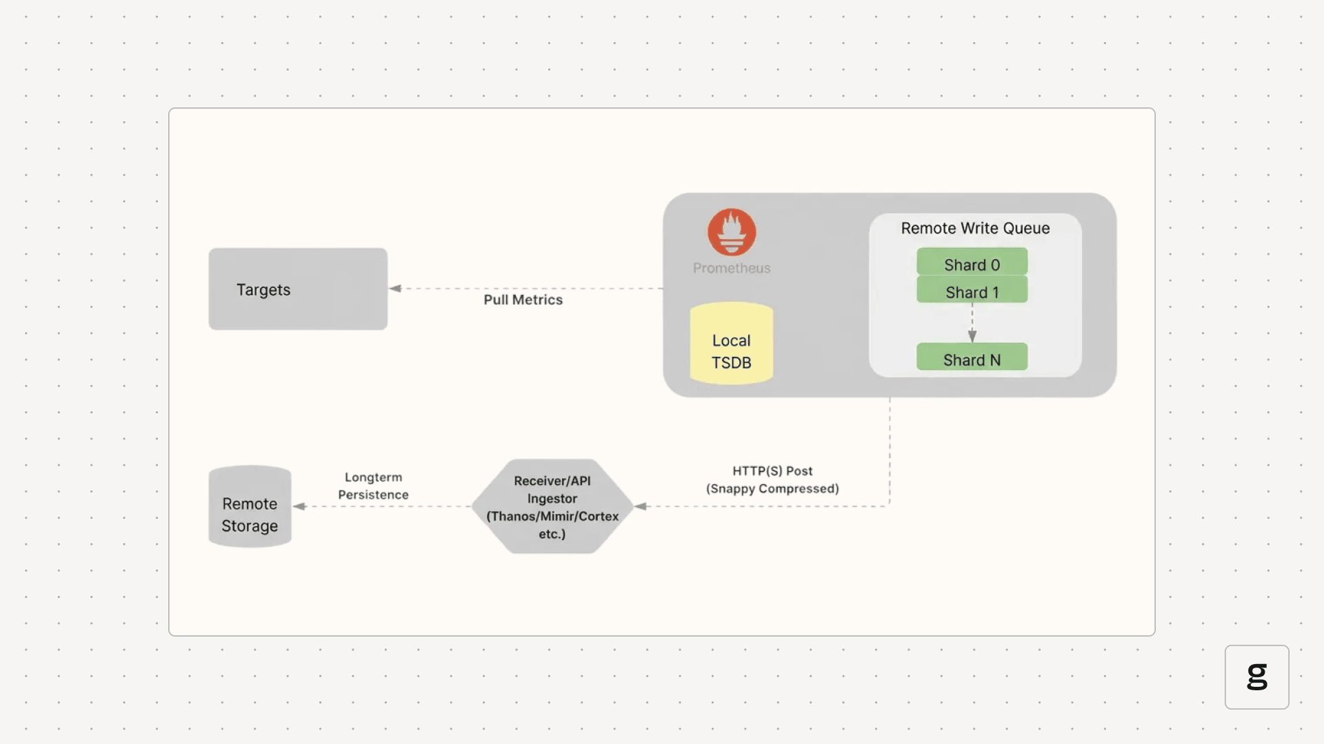
Why Remote Write?
- Long-Term Storage: Local Prometheus TSDBs are typically optimized for short-term retention (e.g., 15 days). Remote Write enables archiving years of data in cloud storage.
- Global View: Consolidate metrics from multiple clusters into a single centralized hub (e.g., Grafana pointing to a central Cortex/Mimir instance).
- High Availability: Feed data into distributed systems built for resilience.
Mechanism: Sharding & Queues
To handle high throughput, Remote Write uses an in-memory queue managed by concurrent shards (worker threads).
- Data Ordering: Samples for the same unique time series are always routed to the same shard to ensure correct ingestion order.
- Retry Logic: Shards implement exponential backoff to handle transient network issues or remote endpoint errors.
4. Federated Observability: Cortex
Cortex is a horizontally scalable, highly available, multi-tenant, long-term storage for Prometheus. It is built as a set of microservices.
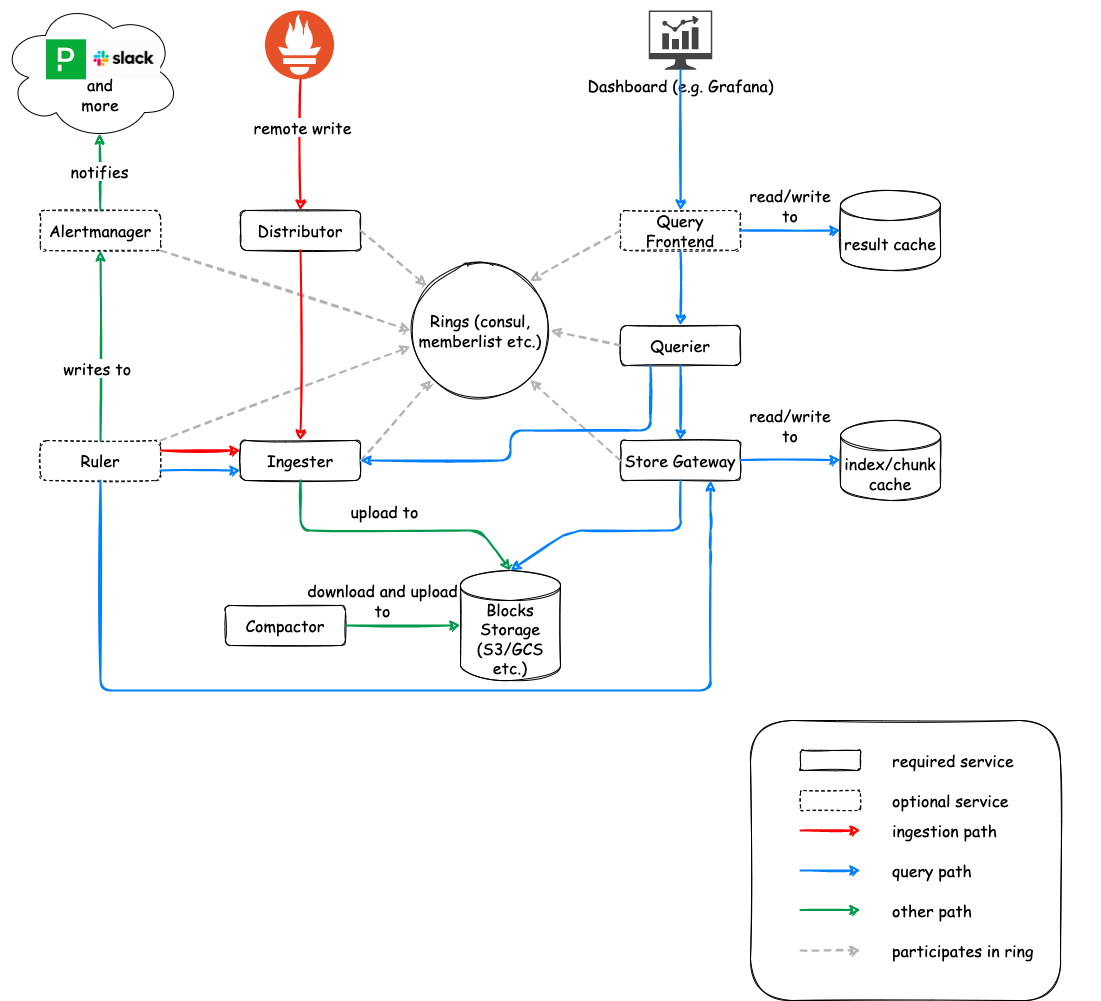
Key Microservices
- Distributor: Handles incoming samples.
- Consistent Hashing: Uses a “hash ring” to route data to the correct Ingesters.
- HA Tracker: Deduplicates samples from redundant Prometheus pairs by tracking leader status via
clusterandreplicalabels. - Quorum Writes: Ensures durability by waiting for a majority of Ingesters to acknowledge the write.
- Ingester: Statefully caches incoming samples in memory.
- WAL (Write Ahead Log): Records data before caching to prevent loss during crashes.
- Chunking: Flushes data blocks to long-term storage (S3, GCS, Azure Blob) once they reach a certain size or age.
- Querier: Executes PromQL queries by fetching data from both Ingesters (for recent data) and long-term storage (via Store Gateway).
Summary: The Metrics Pipeline
- Kubernetes Components: Emit metrics via
/metrics(e.g., Kubelet, API Server). - Enrichment:
kube-state-metricsadds context about object status. - Logs: Nodes use agents like Fluent Bit to forward logs to central stores (e.g., Loki).
- Traces: OpenTelemetry (OTLP) standardized spans are processed via OTel Collectors and stored in backends like Tempo or Jaeger.
References:
Concepts
AI Inference
AI Inference Fundamentals
Efficiently serving Large Language Models (LLMs) requires specialized techniques to overcome memory bottlenecks and maximize throughput.
KV Cache (Key-Value Cache)
In autoregressive decoding, each generated token depends on all previous tokens. To avoid recomputing the attention “keys” and “values” for every new token, they are stored in GPU memory.
- Large: Can take gigabytes for long sequences (e.g., ~1.7GB for a 13B model at 2048 tokens).
- Dynamic: Sizes change based on sequence length, leading to memory management challenges.
- The Problem: Traditional systems over-reserve memory for the maximum possible sequence length (Internal Fragmentation) or fail to reclaim gaps (External Fragmentation), losing 60-80% of actual GPU capacity.
Time to First Token (TTFT)
TTFT is the latency between request submission and the first output token. It is the most critical metric for interactive user experience.
Prefill Phase (Compute-Bound)
The model processes the entire input prompt at once to populate the KV cache. This phase is limited by the GPU’s TFLOPS (compute capacity).
Decoding Phase (I/O-Bound)
Tokens are generated one by one. Each step requires loading the model weights and the KV cache from VRAM to the processors. This phase is limited by Memory Bandwidth.
[!TIP] Optimizing TTFT involves minimizing queuing delays and using efficient “Chunked Prefill” to balance prompt processing with ongoing token generation.
Last updated: 2026-03-25
vLLM & PagedAttention
vLLM is a high-throughput LLM serving engine. Its “secret sauce” is PagedAttention, an algorithm inspired by virtual memory paging in operating systems.
The PagedAttention Mechanism
Instead of allocating contiguous memory for a sequence’s KV cache (which leads to fragmentation), PagedAttention partitions it into fixed-size physical blocks.
Logical vs. Physical Mapping
Contiguous logical blocks of a sequence are mapped to non-contiguous physical blocks via a Block Table. Physical blocks are allocated strictly on demand.
 Animation showing how logical KV cache blocks are mapped to non-contiguous physical memory.
 The PagedAttention kernel fetches blocks efficiently by consulting the Block Table during computation.
Memory Sharing & Copy-on-Write
PagedAttention naturally enables efficient memory sharing for complex sampling algorithms (e.g., parallel sampling, beam search).
- Shared Prompt: Multiple output sequences from the same prompt can point to the same physical blocks.
- Copy-on-Write (CoW): When a shared block needs to be modified, a new physical block is allocated only for the delta.
 Sharing the prompt’s KV cache across multiple generation sequences.
[!NOTE] vLLM reduces memory waste to under 4%, allowing for significantly larger batch sizes and up to 24x higher throughput than standard Transformers implementations.
Last updated: 2026-03-25
Inference Parallelism
When a model is too large for a single GPU or when scaling throughput is required, various parallelism strategies are employed.
Tensor Parallelism (TP)
Shards model weights (tensors) across multiple GPUs within a single layer.
- Scope: Usually within a single node (using high-speed NVLink).
- vLLM Config:
--tensor-parallel-size 4

Pipeline Parallelism (PP)
Distributes different layers of the model across different GPUs.
- Scope: Can span multiple nodes.
- vLLM Config:
--pipeline-parallel-size 2

Data Parallelism (DP)
Replicates the entire model across multiple GPU sets. Each set processes a different batch of requests.
- Best for: Maximizing overall system throughput.

Expert Parallelism (EP)
Used for Mixture-of-Experts (MoE) models (like DeepSeek or Mixtral). It shards the “expert” layers across GPUs while keeping common layers replicated or sharded via TP.

Last updated: 2026-03-25
Distributed Inference Tools
Modern stacks extend beyond simple model servers to include Kubernetes-native orchestration and intelligent routing.
KubeAI
A Kubernetes operator designed to streamline LLM deployments.
- OpenAI Compatible: Seamlessly integrates with existing LLM apps.
- Autoscaling: Supports “Scale-to-Zero” for cost savings.
- Prefix-Aware Routing: Directs requests to pods that already have the relevant KV cache.
- KubeAI.org

LLM-D (LLM Deployer)
A high-performance stack focusing on Disaggregated Serving.
PD Disaggregation
Separates the Prefill (prompt processing) and Decode (token generation) stages into distinct clusters.
- Prefill Clusters: Optimized for high-compute (TFLOPS).
- Decode Clusters: Optimized for high memory bandwidth and low latency.

Tiered KV Caching
LLM-D supports offloading KV-cache entries to:
- CPU RAM: Fast retrieval for warm requests.
- SSD: Persistent storage for long-tail cache.
- Network Storage: Shared cache across nodes.
Last updated: 2026-03-25
Concepts
DevOps: CI/CD Fundamentals
CI/CD Fundamentals
Automation is the engine behind DevOps. CI/CD pipelines provide a reliable, repeatable path for software to move from a developer’s machine to the end-user.
Continuous Integration (CI)
CI focuses on the early stages of the development cycle, ensuring that code changes are integrated and tested frequently.
The CI Workflow
- Code Commit: Developers push code to a shared repository (Git).
- Automated Build: The build server (GitHub Actions, GitLab CI, Jenkins) compiles the code and builds artifacts (Docker images, binaries).
- Static Analysis: Tools like SonarQube or checkstyle analyze code for security vulnerabilities and style issues.
- Testing:
- Unit Tests: Testing individual functions/classes.
- Integration Tests: Testing interactions between components.
- Security (SAST): Scanning source code for vulnerabilities.
Continuous Delivery vs. Deployment (CD)
While often used interchangeably, there is a key distinction in the level of automation.
Continuous Delivery
The code is always in a deployable state. However, the final push to production requires a manual trigger.
- Promotion: Promoting artifacts through staging/QA environments before production.
- Why?: Business requirements, compliance, or risk management.
Continuous Deployment
Every change that passes the automated pipeline is automatically deployed to production.
- Prerequisite: Extremely high confidence in automated testing and observability.
- Benefit: Minimum time-to-market and rapid feedback loops.
Pipeline Design Best Practices
- Build Once, Deploy Many: The same artifact (Docker image) should move through all environments to ensure consistency.
- Fail Fast: Run the fastest, most critical tests first to provide immediate feedback.
- Immutable Artifacts: Never modify an artifact after it’s built; version it and promote it.
- Artifact Management: Use registries like Harbor, Nexus, or JFrog Artifactory to store and version your builds.
| Stage | Goal | Tool Examples |
|---|---|---|
| Source | Version control | Git, GitHub, GitLab |
| Build | Compilation & Packaging | Maven, Go Build, Docker |
| Test | Quality & Security | Jest, JUnit, SonarQube |
| Release | Artifact storage | Harbor, ECR, Nexus |
| Deploy | Orchestration | Kubernetes, Helm, Terraform |
Last updated: 2026-03-25
Concepts
DevOps: Deployment Strategies
Deployment Strategies
Modern software delivery requires strategies that minimize downtime and blast radius. Beyond standard rolling updates, progressive delivery techniques allow for safer, metrics-driven releases.
Core Strategies
Blue/Green Deployment
Two identical environments (Blue=Stable, Green=New).
- Traffic Shifting: Managed at the load balancer or DNS level.
- DB Migrations: The biggest challenge. Strategies include:
- Expand and Contract: First add new columns (expand), then deploy code that uses both, then remove old columns (contract).
- Read-only mode: Briefly put the app in read-only during the switch.
- Pros: Instant rollback by switching back to Blue.
Canary Deployment
Incremental traffic shifting.
- Header-based Routing: Route only internal users or specific regions using HTTP headers (e.g.,
x-user-type: beta). - Automated Analysis: Tools like Argo Rollouts or Flux Flagger automatically compare metrics (Success Rate, Latency) between stable and canary.
- Rollback: Automatically triggered if error rates exceed a threshold.
Rolling Update
The default Kubernetes strategy.
- maxSurge: How many extra pods can be created during the update.
- maxUnavailable: How many pods can be taken down during the update.
- Readiness Probes: Critical for ensuring traffic only hits “warm” and healthy instances.
Recreate
- Usage: When the application cannot handle two versions running simultaneously (e.g., exclusive file locks or complex singleton states).
- Downtime: Scaled by the speed of startup/shutdown.
Progressive Delivery Tools
- Argo Rollouts: A Kubernetes controller that provides advanced deployment capabilities (Blue/Green, Canary, Analysis).
- Istio/Linkerd: Service meshes that enable fine-grained traffic splitting (e.g., 99% vs 1%).
- Feature Flags: Decoupling deployment from release. Code is deployed but hidden behind a toggle (LaunchDarkly, Unleash).
| Strategy | Speed | Risk | Seamless | Complexity |
|---|---|---|---|---|
| Recreate | Fast | High | No | Low |
| Rolling | Slow | Medium | Yes | Low |
| Blue/Green | Fast | Low | Yes | High |
| Canary | Slow | Lowest | Yes | High |
Last updated: 2026-03-25
Concepts
DevOps: IaC & GitOps
Infrastructure as Code (IaC) & GitOps
Treating infrastructure like software is the cornerstone of modern DevOps. This ensures reproducibility, auditability, and speed.
Infrastructure as Code (IaC)
IaC allows teams to manage and provision infrastructure through code rather than manual processes.
Key Concepts
- Declarative vs Imperative:
- Declarative: Focuses on the desired state (e.g., “I want 3 VMs”). Examples: Terraform, OpenTofu, CloudFormation, Pulumi.
- Imperative: Focuses on the steps to achieve the state (e.g., “Run this script to install Nginx”). Examples: Ansible, Chef, Puppet.
- Idempotency: The ability to run the same code multiple times and achieve the same result without unintended side effects.
- State Management: Tools like Terraform maintain a
.tfstatefile to track the real-world resources and map them to your code.
Terraform Deep Dive
- Providers: Plugins that interact with cloud APIs (AWS, GCP, Kubernetes).
- Modules: Reusable building blocks to standardize infrastructure patterns.
- Backends: Remote storage for state files (S3, GCS, Terraform Cloud) with locking mechanisms (DynamoDB) to prevent concurrent changes.
GitOps Principles
GitOps is an operational framework that takes DevOps best practices (version control, collaboration, CI/CD) and applies them to infrastructure automation.
The Four Pillars
- Declarative Description: The entire system is described declaratively in Git.
- Versioned Source of Truth: Changes to the system are made via Pull Requests.
- Automatically Pulled: The infrastructure is automatically updated when the Git state changes.
- Continuously Reconciled: Software agents (operators) constantly compare the desired state (Git) with the actual state (Cluster).
GitOps vs Traditional CI/CD
| Feature | Traditional CD (Push) | GitOps (Pull) | | :— | :— | :— | | Trigger | CI server pushes to Cluster | Cluster agent pulls from Git | | Security | CI needs cluster credentials | Agents run inside the cluster | | Drift | Hard to detect | Automatically corrected |
Tools
- ArgoCD: Provides a powerful UI and supports multi-cluster management.
- Flux CD: A lightweight, CNCF-graduated tool focused on automation and security.
- Sealed Secrets / External Secrets: Strategies to manage sensitive data in Git without storing plan-text secrets.
| Tool | Focus | Philosophy |
|---|---|---|
| Terraform | Infrastructure Provisioning | Generic, multi-cloud |
| Ansible | Configuration Management | Procedural, agentless |
| ArgoCD | Kubernetes CD | GitOps, UI-driven |
Last updated: 2026-03-25
Concepts
DevOps: Git Internals
Git Internals & Advanced Config
Git is a content-addressable filesystem. Understanding how it moves data between its internal areas is key to mastering the tool.
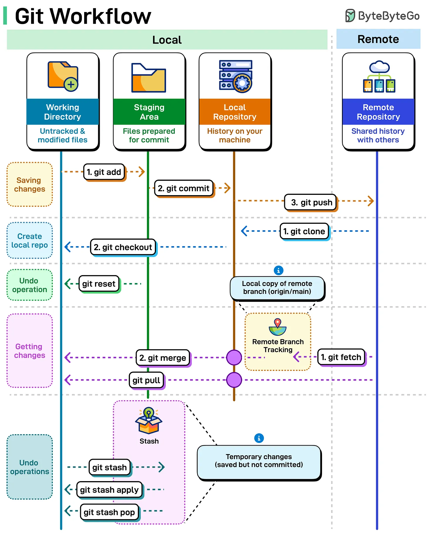
The Git Workflow (4 Areas)
Git manages your code across four distinct areas. Most commands are simply moving data between these stages.
- Working Directory: Your local files on disk that you are currently editing.
- Staging Area (Index): A “draft” area where you prepare changes for the next commit.
- Local Repository (HEAD): Your personal version history on your machine.
- Remote Repository: The shared version of the project (e.g., GitHub, GitLab).
Essential Commands
git add: Moves changes from Working Directory to Staging Area.git commit: Saves staged changes to the Local Repository.git push: Uploads local commits to the Remote Repository.git fetch: Downloads updates from Remote to Local Repository (without merging).git merge: Integrates downloaded changes into your current branch.git pull: Performsfetch+mergein a single step.git checkout: Switches between branches or restores files.git stash: Temporarily “shelves” changes in the Working Directory to be restored later.
Visualizing the Data Flow
Advanced Configurations
These settings are frequently used by Git core developers to improve the default experience, focusing on better diffing, pushing, and conflict resolution.
Better Diffing & Visibility
# Use the smarter histogram diff algorithm
git config --global diff.algorithm histogram

# Highlight moved code in different colors
git config --global diff.colorMoved plain

# Show the full diff when writing commit messages
git config --global commit.verbose true
Streamlined Pushing & Fetching
# Automatically set upstream branch on first push
git config --global push.autoSetupRemote true

# Automatically prune stale remote-tracking branches on fetch
git config --global fetch.prune true

# Push tags automatically when pushing branches
git config --global push.followTags true
Conflict Resolution & Maintenance
# Show the "base" version in merge conflicts (Zealous Diff3)
git config --global merge.conflictstyle zdiff3

# Reuse recorded resolutions (rerere) for repeating conflicts
git config --global rerere.enabled true
git config --global rerere.autoupdate true

# Default to rebase when pulling
git config --global pull.rebase true

# enable filesystem monitor for faster status in large repos
git config --global core.fsmonitor true
Safety & Automation
# Guess and prompt for autocorrecting mistyped commands
git config --global help.autocorrect prompt

# Automatically stash/pop changes before/after rebase
git config --global rebase.autoStash true
Sources:
Last updated: 2026-03-25
Concepts
DevOps: Linux Fundamentals
Understanding the Linux Directory Structure
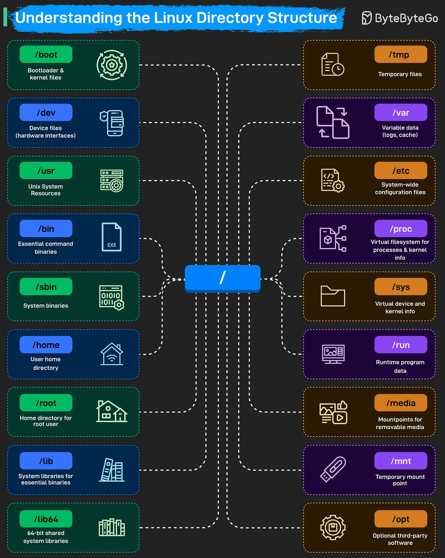
The Linux filesystem follows a hierarchical structure, starting from the root directory /. Everything in Linux—including hardware devices, processes, and system configurations—is represented as a file within this tree.
The Linux Filesystem Hierarchy
Core System Directories
/(Root): The starting point of the entire filesystem. Every other directory is a child of root./boot: Stores the bootloader (e.g., GRUB) and kernel files. The system cannot start without this directory./bin&/sbin: Contain essential binaries and system commands./binholds commands for all users, while/sbinholds system administration binaries./lib&/lib64: System libraries that support the binaries in/binand/sbin.
Configuration & Data
/etc: The central location for all system-wide configuration files./home: Contains personal directories for regular users (e.g.,/home/alice)./root: The home directory for the root (superuser) account./var: Stores “variable” data that changes frequently, such as logs (/var/log), caches, and spool files./tmp: A place for temporary files, which are often cleared on reboot.
Resources & Applications
/usr: Contains user-level applications, libraries, and source code. It is often the largest directory on the system./opt: Reserved for “optional” or third-party software packages (e.g., Chrome, Zoom)./run: Records runtime information for programs since the last boot (e.g., PID files).
Hardware & Virtual Filesystems
/dev: Holds device files that act as interfaces to hardware (e.g.,/dev/sdafor a disk)./proc: A virtual filesystem that provides information about running processes and kernel parameters./sys: Another virtual filesystem that exposes kernel information about hardware devices and drivers./media&/mnt: Used for mounting external storage./mediais typically for auto-mounted removable devices (USB, CD-ROM), while/mntis for manual temporary mounts.
Source: ByteByteGo - Understanding the Linux Directory Structure
Last updated: 2026-03-25
The Linux Boot Process Explained
Understanding how a Linux system starts up is fundamental for system administration and troubleshooting. The process involves a sequence of handovers from hardware firmware to the operating system kernel and finally to user-space services.
The 8 Stages of Linux Boot
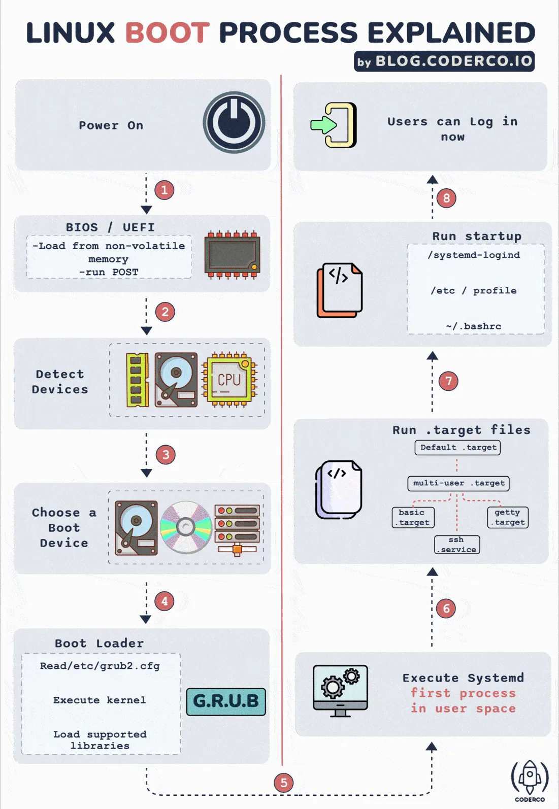
1. BIOS / UEFI
When the power is turned on, the BIOS (Basic Input/Output System) or UEFI (Unified Extensible Firmware Interface) is loaded from non-volatile memory. It performs a POST (Power-On Self-Test) to ensure the hardware is functioning correctly.
2. Hardware Detection
The firmware detects connected devices, including the CPU, RAM, and storage controllers, preparing the system for the next stage.
3. Boot Device Selection
The system looks for a bootable device based on a predefined priority (e.g., Hard Drive, NVMe, Network/PXE, or USB).
4. Bootloader (GRUB)
The firmware loads and executes the bootloader (commonly GRUB - GRand Unified Bootloader). GRUB provides a menu to select the OS/Kernel and loads the chosen Kernel and initramfs (initial RAM filesystem) into memory.
5. Kernel Initialization
The Linux kernel takes control. It initializes hardware drivers, mounts the root filesystem (often using initramfs as a temporary bridge), and starts the first user-space process: systemd (PID 1).
6. Systemd (The Init System)
systemd manages system services and processes. It probes remaining hardware, mounts the final filesystems, and works toward reaching the default.target (usually a multi-user or graphical environment).
7. Target Configuration
The system executes startup scripts and configures the environment according to the active target unit (comparable to traditional “runlevels”).
8. User Login
Once all services are active, the system presents a login prompt or a desktop environment. The boot process is complete.
Linux Boot vs. Cloud-Init Boot
In cloud environments (AWS, GCP, Azure), the standard boot process is extended by cloud-init to handle dynamic configuration (metadata, SSH keys, networking).
| Stage | Standard Linux Boot | Cloud-Init Extension |
|---|---|---|
| Early Boot | Kernel starts systemd. | systemd-generator detects the cloud environment and enables cloud-init. |
| Local | System waits for storage/network local configs. | cloud-init-local: Searches for datasources (metadata) and applies network configuration before networking is even up. |
| Network | Networking services start. | cloud-init-network: Processes user-data (e.g., mounting disks) now that the network is available. |
| Config | Standard services start. | cloud-init-config: Runs configuration modules like SSH keys, user creation, and package mirrors. |
| Final | User login prompt appears. | cloud-init-final: Runs late-stage tasks like package installations and user-provided scripts (bootcmd). |
Key Differences
- Purpose: Standard boot focuses on getting the OS running;
cloud-initfocuses on provisioning and customizing the instance. - Dynamic Data: Standard boot is relatively static.
cloud-initconsumes external metadata and user-data at runtime to configure the machine. - Idempotency: Standard boot runs every time.
cloud-inittypically runs its heavy configuration logic only on the first boot of an instance.
Sources: ByteByteGo - Linux Boot Process, CoderCo - The Linux Boot Process
Last updated: 2026-03-26
Network Troubleshooting Test Flow
Most network issues look complicated, but the troubleshooting process doesn’t have to be. A reliable way to diagnose problems is to test the network layer by layer, starting from your own machine and moving outward until you find exactly where things break.
Troubleshooting Workflow
The following flow provides a structured checklist that mirrors how packets actually move through a system.
graph TD
    Start([Start]) --> LocalCheck[Local System Check<br/>Test TCP/IP stack & NIC status]

    LocalCheck --> PingLocal{ping 127.0.0.1<br/>& Verify NIC enabled}
    PingLocal -- NO --> FixLocal[Fix TCP/IP / Enable NIC]
    FixLocal --> PingLocal
    PingLocal -- YES --> LocalIP[Test Local IP Configuration<br/>Check local IP & self-connectivity]

    LocalIP --> PingSelf{Verify DHCP/Static IP<br/>+ ping self IP}
    PingSelf -- NO --> FixIP[Fix DHCP / IP config / firewall]
    FixIP --> PingSelf
    PingSelf -- YES --> LAN[Test LAN Connectivity<br/>Check LAN gateway reachability]

    LAN --> PingGW{ARP resolution +<br/>ping default gateway}
    PingGW -- NO --> FixLAN[Fix cable / switch / IP conflict]
    FixLAN --> PingGW
    PingGW -- YES --> Routing[Test Internal Routing]

    Routing --> PingExit{Check default route +<br/>ping exit router}
    PingExit -- NO --> FixRoute[Fix routing table / router uplink / ACL]
    FixRoute --> PingExit
    PingExit -- YES --> WAN[Test ISP/WAN Connectivity<br/>Verify WAN link & ISP gateway]

    WAN --> PingWAN{Check WAN interface IP +<br/>ping ISP gateway}
    PingWAN -- NO --> FixWAN[Fix DHCP/PPPoE/modem/ONT/NAT/ISP]
    FixWAN --> PingWAN
    PingWAN -- YES --> Internet[Test Internet Connectivity<br/>Check external Internet reachability]

    Internet --> PingPublic{ping 8.8.8.8<br/>public DNS IP}
    PingPublic -- NO --> FixInternet[Fix upstream routing / ISP issues]
    FixInternet --> PingPublic
    PingPublic -- YES --> DNS[DNS Resolution]

    DNS --> NSLookup{nslookup or dig<br/>domain name}
    NSLookup -- NO --> FixDNS[Fix DNS server config / change DNS]
    FixDNS --> NSLookup
    NSLookup -- YES --> Target[Test Target & Application<br/>Check target host & service]

    Target --> PingTarget{ping target IP +<br/>test TCP port}
    PingTarget -- NO --> FixTarget[Fix server / ICMP / firewall / service / port]
    FixTarget --> PingTarget
    PingTarget -- YES --> OK([NETWORK OK!])

    style Start fill:#f9f,stroke:#333,stroke-width:2px
    style OK fill:#0f0,stroke:#333,stroke-width:2px
    style FixLocal fill:#f66,stroke:#333,stroke-width:1px
    style FixIP fill:#f66,stroke:#333,stroke-width:1px
    style FixLAN fill:#f66,stroke:#333,stroke-width:1px
    style FixRoute fill:#f66,stroke:#333,stroke-width:1px
    style FixWAN fill:#f66,stroke:#333,stroke-width:1px
    style FixInternet fill:#f66,stroke:#333,stroke-width:1px
    style FixDNS fill:#f66,stroke:#333,stroke-width:1px
    style FixTarget fill:#f66,stroke:#333,stroke-width:1px
Step-by-Step Breakdown
1. Local System Check
Ensure your computer’s networking stack is functioning.
- Action:
ping 127.0.0.1(loopback address) and check if the Network Interface Card (NIC) is enabled. - Troubleshooting: If this fails, the issue is likely software (TCP/IP stack corruption) or hardware (NIC disabled/broken).
2. Test Local IP Configuration
Verify that your machine has a valid IP address and can talk to itself.
- Action: Check your IP (e.g.,
ip addrorifconfig) andpingyour own IP. - Troubleshooting: Check DHCP settings, static IP configurations, or local firewall rules blocking self-connectivity.
3. Test LAN Connectivity
Check if you can reach other devices on your local network.
- Action:
pingyour default gateway (usually your router’s IP). Checkarp -ato see if MAC addresses are resolving. - Troubleshooting: Check cables, network switches, or look for IP address conflicts on the subnet.
4. Test Internal Routing
Verify that packets can leave the local subnet properly.
- Action: Check your routing table (
ip route) andpingthe next-hop router if applicable. - Troubleshooting: Fix incorrect static routes, check router uplinks, or check Access Control Lists (ACLs).
5. Test ISP/WAN Connectivity
Confirm the connection to your Internet Service Provider.
- Action: Check the external WAN interface IP and
pingthe ISP’s gateway. - Troubleshooting: Check the modem, ONT (Optical Network Terminal), or PPPoE/DHCP status with the ISP.
6. Test Internet Connectivity
Verify if you can reach a known stable IP on the public Internet.
- Action:
ping 8.8.8.8(Google’s Public DNS) or1.1.1.1(Cloudflare). - Troubleshooting: Issues here usually point to upstream routing problems or ISP-wide outages.
7. DNS Resolution
Confirm that domain names are being translated into IP addresses.
- Action:
nslookup google.comordig google.com. - Troubleshooting: Update
/etc/resolv.conf, check local DNS cache, or switch to a different DNS provider (e.g., Google or Cloudflare).
8. Test Target & Application
Check if the specific target server and service are available.
- Action:
ping <target_ip>and test the specific service port (e.g.,telnet <ip> 80ornc -zv <ip> 443). - Troubleshooting: The target server might be down, ICMP might be blocked by a firewall, or the application service (port) might not be running.
Source: ByteByteGo - Network Troubleshooting Test Flow
Last updated: 2026-03-25
Linux Internals: The SRE Safety Net
When engineers ask about “Linux Internals,” they are often testing whether you understand how the OS affects your application performance. You don’t need to memorize the kernel source code; you just need to know where the “knobs” are and how to interpret common metrics.
Linux Server Review (The ‘SadServers’ Way)
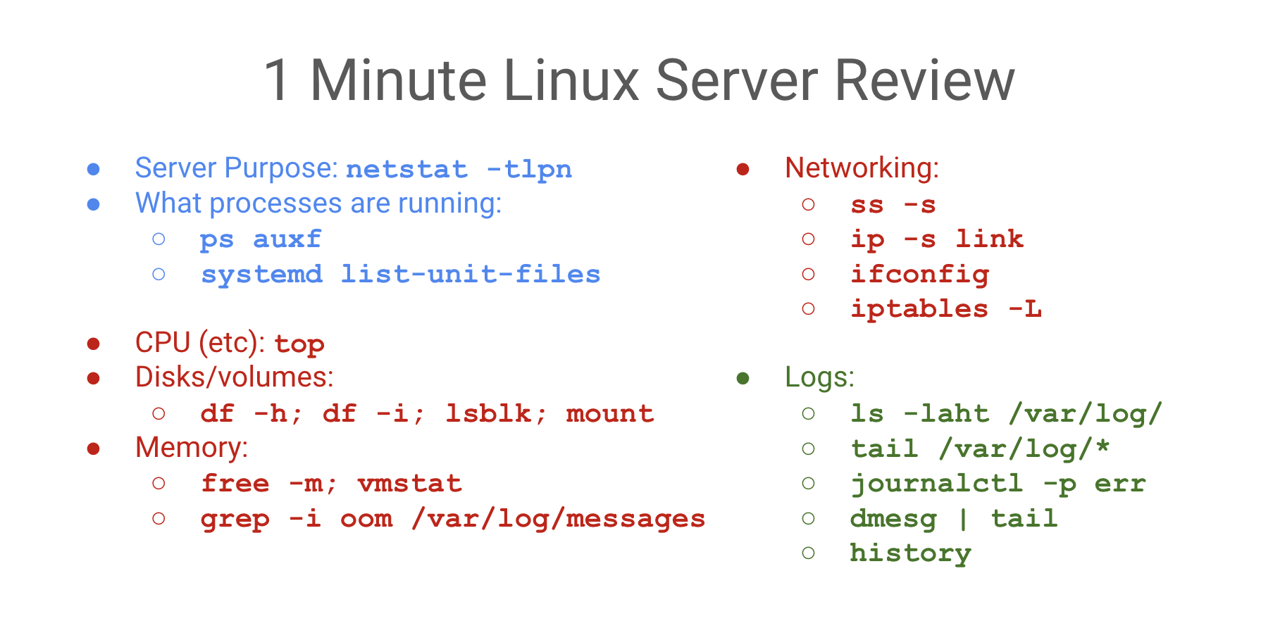
The “Safety Net” Logic
If a process is slow or crashing, the problem is almost always one of these four: CPU, Memory, Disk (I/O), or Network.
1. Quick Triage (Load & Basics)
uptime: Check load averages (1, 5, 15 min). Load > # of cores = saturation.top/htop: Real-time view of processes and resource consumers.ps auxf: Process tree;fshows parent/child relationships (useful for identifying worker leaks).uname -a&cat /etc/debian_version: Quick check of kernel and distro version.
2. CPU & Performance
mpstat -P ALL 1: Check CPU balance. Are all cores busy, or just one (single-threaded bottleneck)?pidstat 1: Per-process CPU usage. Identify which PID is specifically spiking.lscpu: Verify CPU architecture and core count.
3. Memory & Virtual Memory
free -m: Quick overview of used/cached/free memory.vmstat 1: Checkr(runnable) andb(uninterruptible sleep/disk wait). Highsi/someans swapping!grep -i oom /var/log/syslog: Check if the OOMKiller has been active recently.
Virtual vs. Physical Memory (VIRT vs. RSS)
- VIRT (Virtual Memory): The absolute total memory a process can “see”. It includes shared libraries, swapped out pages, and memory requested via
malloc()but not yet used. - RSS (Resident Set Size): The actual amount of physical RAM the process is using right now.
- Lazy Allocation (Demand Paging):
- When a process calls
malloc(), the kernel gives it Virtual Memory (VIRT increases). It’s just a “promise” of space. - The kernel only allocates Physical Memory (RSS increases) when the process actually touches the address (reads or writes).
- This first touch triggers a Page Fault, and the kernel then maps a real physical page to that virtual address.
- When a process calls
4. Disk & I/O
df -h: Check for full filesystems. 100% disk = certain failure for most apps.df -i: Check for Inode exhaustion. You can have GBs free but 0 inodes.iostat -xz 1: Check%util. If a disk is at 100% util, it’s the bottleneck.lsblk -f: List block devices and their filesystems.du -mxS / | sort -n | tail -10: Find the top 10 largest files in a directory.
5. Networking & Connectivity
ss -tlpn: (Socket Stat) What processes are listening on which ports?ss -s: Summary of socket statistics (TCP/UDP/ESTAB).ip -s link: Check for interface errors or dropped packets.netstat -i: Network interface statistics.iptables -L -n -t nat: Check firewall and NAT rules (don’t forget-t natfor K8s/Docker!).
6. Logs & systemd
journalctl -xe: View the most recent system logs with explanations.journalctl -u nginx: View logs for a specific service.journalctl -k: View kernel messages (equivalent todmesg).systemctl --failed: List all units that failed to start.systemd-analyze blame: See which services are making boot-up slow.
7. Isolation & Namespaces (Boundaries)
Namespaces define what a process can see. They create isolated views of system resources.

- PID Namespace: The process thinks it is PID 1.
- Network Namespace: Private network stack (interfaces, routing, IP).
- Mount Namespace: Independent filesystem mount points.
- UTS Namespace: Custom hostname.
- IPC Namespace: Isolated inter-process communication.
- User Namespace: Map internal IDs to different external IDs (e.g., internal root = external nobody).
Control Groups (cgroups)
Cgroups define how much a process can use. They enforce resource limits (CPU, Memory, I/O) and prevent “noisy neighbors” from starving other processes.
4. Virtual File System (VFS) & Storage
Linux treats “everything as a file” via the VFS abstraction layer.
Inodes (The File’s Identity)
An Inode is a data structure containing metadata about a file (permissions, owner, size, data block addresses).
- Crucial Fact: The Filename is NOT stored in the Inode. It’s stored in the directory entry that points to the Inode.
- Links: A Hard Link is just another directory entry pointing to the same Inode. A Symlink is a special file containing the path to another Inode.
File Behavior & Inodes
cp(Copy): Creates a NEW Inode.mv(Move): Keeps the SAME Inode (just renames the directory entry pointer).sed -i(Edit in place): Often creates a temporary file (new Inode) and renames it over the original. This can break tools (liketail -f) that are watching the original Inode!
File Descriptors (FD)
A File Descriptor is a process-level integer that index into the kernel’s open file table. By default, 0 is stdin, 1 is stdout, and 2 is stderr.
Sources: SadServers, Dev.to - Linux FS, [ByteByteGo]
Last updated: 2026-03-26
Linux File System & Permissions
In Linux, “everything is a file.” This philosophy is managed through a sophisticated system of metadata and abstraction.
The Inode (Index Node)
An Inode is the data structure that stores all information about a file except its name and the actual data content.
Inode Metadata
You can view this with stat [filename] or ls -i:
- File Type: Regular (-), Directory (d), Symlink (l), etc.
- Permissions: Read, write, execute bits.
- Owner/Group: UID and GID.
- Size: Total bytes.
- Timestamps: Access (atime), Modify (mtime), Change (ctime).
- Blocks: The location of data on the physical disk.
File Permissions
Linux uses a 3-tier permission model: User (u), Group (g), and Others (o).
Octal Representation
- Read (r): 4
- Write (w): 2
- Execute (x): 1
- No Permission: 0
Example: chmod 755 (rwxr-xr-x) means User has 7 (4+2+1), Group/Others have 5 (4+1).
Special Permissions
- SUID (Set User ID): The process runs with the privileges of the file’s owner (e.g.,
/usr/bin/passwd). - SGID (Set Group ID): The process runs with the privileges of the file’s group. In directories, new files inherit the parent’s group.
- Sticky Bit: Applied to directories (like
/tmp) to ensure only the file owner can delete or rename their own files. - SELinux Dot (
.): A dot at the end of permissions (e.g.,-rw-r--r--.) indicates an SELinux security context is active.
Storage & Capacity
Disk Usage Tools
df -h: (Disk Free) Shows the filesystem’s total capacity and remaining space. Best for high-level health checks.du -sh [dir]: (Disk Usage) Traverses a specific directory to calculate size. Best for finding large files.- Difference:
dfreports space used at the filesystem level, whiledureports the sum of file sizes. If you delete a large file that a process still has open,duwill show the space as free, butdfwill show it as still used!
File System Types
You can check active filesystems with df -T, lsblk -f, or mount.
- ext4: 4th Extended Filesystem (Standard).
- xfs: High-performance journaling filesystem (Default in RHEL/CentOS).
- tmpfs: RAM-backed filesystem (Volatile).
Last updated: 2026-03-26
Linux Process Management
Processes are executing instances of a program, each with its own memory space and resources.
Process Lifecycle
Every process in Linux is created by another process (except PID 1, which is started by the kernel).
fork(): A parent process creates a near-identical copy of itself.exec(): The child process replaces its memory space with a new program.exit()/wait(): The process finishes and its parent collects its exit status.
Zombies vs. Orphans
- Zombie Process (
Z): A process that has finished execution but still occupies an entry in the process table because its parent hasn’t yet “reaped” it viawait(). - Orphan Process: A process whose parent has died. These are automatically adopted by PID 1 (
systemdorinit).
Process States
You can see these in top or ps:
R(Running / Runnable): Actively using the CPU or waiting in the run queue.S(Interruptible Sleep): Waiting for an event (e.g., user input).D(Uninterruptible Sleep): Waiting for I/O (e.g., disk access). Cannot be killed until I/O finishes.T(Stopped): Suspended by a signal (e.g.,Ctrl+Z).Z(Zombie): Terminated but still in the process table.
Signals
Signals are a way to send messages to processes.
SIGTERM(15): The default “clean” shutdown. Asks the process to exit.SIGKILL(9): Forcibly kills the process. Cannot be ignored or caught.SIGHUP(1): Hangup. Often used to tell a daemon to reload its configuration without restarting.SIGINT(2): Interrupt (usuallyCtrl+C).SIGSTOP(19): Stops a process (usuallyCtrl+Z).
Monitoring & Troubleshooting
System Load (uptime)
The Load Average represents the number of processes that are either in the R (Running) or D (Uninterruptible) state.
- A load of 1.0 on a 1-core machine means the CPU is at 100% capacity.
- A load of 5.0 on a 4-core machine means the system is over-saturated (1 process is always waiting).
Debugging with strace
strace intercepts and records the system calls (syscalls) made by a process. Use it to find “why” a process is failing (e.g., “File not found” or “Permission denied” at the kernel level).
strace -p [PID] # Attach to a running process
strace ls /root # See what syscalls 'ls' makes
Last updated: 2026-03-26
Linux Interview Preparation
A collection of common technical questions and “under the hood” explanations for Linux system administration.
“What happens when you run ls *.txt?”
This tests your understanding of Shell Expansion vs. the command itself.
- Wildcard Expansion: The shell (e.g., Bash) scans the current directory and replaces
*.txtwith a list of matching filenames (e.g.,a.txt,b.txt). - Execution: The shell then executes the
lscommand, passing the expanded list as arguments:ls a.txt b.txt. - Result:
lsreceives the filenames, not the*symbol.
Kernel & Modules
- How do you find the kernel version?:
uname -roruname -a. - How do you load a kernel module?:
modprobe [module_name]. (Uselsmodto see loaded modules). - What is
sysctl?: A tool used to modify kernel parameters at runtime.- Example:
sysctl -w net.ipv4.ip_forward=1(Enables IP forwarding). - Persist configuration in:
/etc/sysctl.conf.
- Example:
User Limits (ulimit)
The ulimit command defines the resources a user shell can consume.
- Soft Limit: A warning threshold (can be increased by the user up to the hard limit).
- Hard Limit: An absolute ceiling (can only be increased by root).
- Common metric:
ulimit -n(Maximum number of open file descriptors).
The “Everything is a File” Philosophy
In Linux, devices, sockets, and processes are represented as files in the tree:
/dev/sda: The physical hard drive./proc/meminfo: A virtual “window” into the kernel’s memory management./dev/null: The “black hole” used for discarding output (> /dev/null 2>&1).
System Health Checklist
- Characterize:
ss -tlpn(ports),ps auxf(processes). - Saturation:
uptime(load),free -m(memory),df -h(disk). - Errors:
journalctl -p err,dmesg | tail.
Last updated: 2026-03-26
Concepts
DevOps: Docker Fundamentals
Docker Fundamentals
Docker is a platform for building, running, and shipping applications in isolated environments called containers. It provides a consistent environment across development, testing, and production.
Docker Architecture
Docker uses a client-server architecture:
- Docker Daemon (
dockerd): The background process that manages Docker objects like images, containers, networks, and volumes. - Docker Client (
docker): The command-line interface (CLI) used to communicate with the daemon via REST API. - Docker Registries: Storage systems for Docker images (e.g., Docker Hub, GitHub Container Registry).
- Docker Objects:
- Images: Read-only templates used to create containers.
- Containers: Runnable instances of an image.
The Dockerfile
A Dockerfile is a text document containing all the commands a user could call on the command line to assemble an image. It is the “recipe” for creating Docker images.
Key Directives
| Instruction | Description |
|---|---|
FROM | Required. Sets the base image (e.g., FROM node:20-alpine). |
RUN | Executes commands in a new layer (e.g., RUN apt-get update). |
COPY | Copies files/directories from the host to the image. |
ADD | Similar to COPY, but can also handle remote URLs and extract tarballs. |
WORKDIR | Sets the working directory for subsequent instructions (RUN, CMD, etc.). |
ENV | Sets environment variables (persist in the image). |
ARG | Defines variables that users can pass at build-time with --build-arg. |
EXPOSE | Documents which ports the application listens on. |
USER | Sets the user/UID to use when running the image. |
VOLUME | Creates a mount point for persistent data. |
LABEL | Adds metadata to your image (e.g., maintainer, version). |
CMD | Provides defaults for an executing container. Easily overridden by CLI arguments. |
ENTRYPOINT | Configures a container that will run as an executable. Harder to override. |
Building & Managing Images
To create an image from a Dockerfile, use the docker build command:
# Build an image with a tag
docker build -t my-app:v1 .

# List local images
docker images

# Remove an image
docker rmi my-app:v1
Layered Images Explained
Docker images are composed of a series of read-only layers. Each instruction in your Dockerfile that modifies the filesystem (like RUN, COPY, ADD) creates a new layer.
- Immutability: Once a layer is created, it never changes.
- Caching: Docker caches layers to speed up subsequent builds. If a layer hasn’t changed, Docker reuses it.
- Copy-on-Write (CoW): When you run a container, Docker adds a thin read-write layer (“container layer”) on top of the image layers. Any changes made by the running container (creating/deleting files) are stored in this layer.
Visualizing Layers
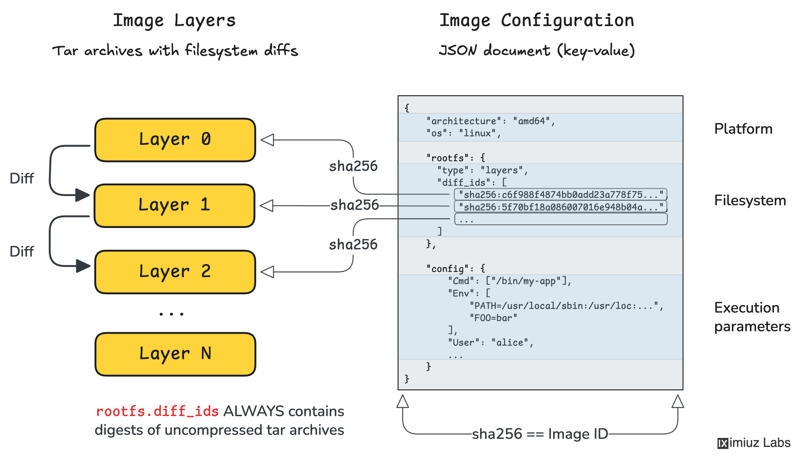
Sources:
Last updated: 2026-03-25
Concepts
DevOps: SRE Principles
Site Reliability Engineering (SRE)
SRE is what happens when you ask a software engineer to design an operations function. It focuses on scalability, reliability, and automation.
Reliability Measurement
The core of SRE is the quantitative measurement of reliability through targets and budgets.
SLI, SLO, and SLA
- SLI (Service Level Indicator): A quantitative measure of some aspect of the service (e.g., Request Latency, Error Rate).
- SLO (Service Level Objective): A target value for an SLI (e.g., 99.9% of requests must be < 200ms).
- SLA (Service Level Agreement): A business-level contract that defines the consequences (e.g., refunds) for meeting or missing SLOs.
Error Budget
An error budget is 1 - SLO. It’s the amount of “unreliability” allowed for a given period.
- Example: A 99.9% SLO allows for ~43 minutes of downtime per month.
- Policy: If the budget is exhausted, releases are halted to focus on improvements.
The Four Golden Signals
Effective monitoring focuses on four key metrics:
- Latency: The time it takes to service a request.
- Traffic: A measure of how much demand is being placed on the system.
- Errors: The rate of requests that fail (explicitly, implicitly, or by policy).
- Saturation: How full your service is (e.g., CPU, Memory, I/O).
Observability Pillars
Observability is more than just monitoring; it’s the ability to understand the internal state of a system from its external outputs.
- Metrics: Aggregated data (counter, gauge, histogram). Best for finding “that” something is wrong.
- Logs: Discrete events. Best for finding “where” something is wrong.
- Traces: End-to-end request flows. Best for finding “why” something is wrong in distributed systems.
Toil and Automation
Toil is the kind of work tied to running a production service that tends to be manual, repetitive, automatable, and devoid of enduring value.
- SRE Target: SREs should spend at least 50% of their time on engineering projects (automation, reliability features) to reduce toil.
| Concept | Purpose |
|---|---|
| Post-mortem | Blameless analysis of an incident to prevent recurrence. |
| Incident Management | Structured process for responding to service disruptions. |
| Capacity Planning | Ensuring the system can handle future loads efficiently. |
Last updated: 2026-03-25
Concepts
Programming: Golang
Golang Fundamentals
A brief overview of the core concepts that define Go’s behavior and performance.
Typing & Data Structures
Arrays vs. Slices
- Arrays: Fixed size, value types. Passing an array to a function copies the entire array.
var a [5]int
- Slices: Dynamic size, reference types (descriptors). They point to an underlying array.
- Internal Structure: Under the hood, a slice is a struct consisting of a pointer (to the first element of the backing array), a
len(current number of elements), and acap(capacity, the maximum elements the slice can hold without reallocating). - Creation: Pre-allocating with
make([]Type, length, capacity)avoids the overhead of implicit reallocations when you know the rough target size. - Growth: Using
appendpushes items to the end. If elements exceed capacity, Go runtime automatically allocates a new larger backing array (often doubling in size), copies existing elements, and updates the slice reference. - Slicing Syntax (
s[low:high]): Creates a new slice that shares the exact same underlying backing array. Adding elements to it can inadvertently overwrite the original slice contents if they overlap. Full-slice expressions[low:high:max]elegantly solves this by constraining the maximum capacity the new slice inherits, safely preventing accidental overwrites.
- Internal Structure: Under the hood, a slice is a struct consisting of a pointer (to the first element of the backing array), a
Maps (Hash Tables)
- Hash tables for key-value pairs. Reference types, initialized using
make(map[keyType]valueType). - Concurrency: Not thread-safe for concurrent writes. Rely on
sync.RWMutexto prevent crashes when simultaneously reading and writing map data. - Nil values: Retrieving an un-set key returns the value type’s global zero-value (e.g.
0,""). Rely on the two-value variant (val, ok := m[key]) to gracefully distinguish missing keys from genuine zero-value assignments. - Internal Structure: Built over an array of buckets (
bmap). Each bucket holds a maximum of 8 key-value records. To expedite iteration, buckets contain atophasharray caching the topmost 8 bits of keys, skipping extensive deep-equal checks. - Collisions & Chaining: If more than 8 elements hash to a single bucket, an overflow bucket pointer is linked.
- Map Growth: Triggered under two circumstances:
- High Load Factor: if average pair count per bucket exceeds 6.5. Runtime doubles bucket count.
- Clustered Overflows: Too many overflow buckets from successive deletions vs insertions. Triggers a same-size growth to de-fragment storage.
- Incremental Evacuation: Expanding maps don’t move records concurrently (to prevent “Stop The World” application freezing). Go performs “Incremental Evacuation”, gently moving records gradually over subsequent regular map operations until all buckets are transferred over seamlessly.
Interfaces
- Implicit implementation (no
implementskeyword). - Defined by a set of methods. Any type that provides those methods satisfies the interface.
- “Accept interfaces, return structs.”
Methods
- Functions with a receiver.
- Value Receiver (
func (v Type) Method()): Works on a copy. - Pointer Receiver (
func (p *Type) Method()): Can modify the original value and avoids copying large structs.
Memory Management & GC
Go handles memory allocation and deallocation automatically.
Stack vs. Heap
- Stack: Used for local variables with predictable lifetimes. Very fast allocation/deallocation.
- Heap: Used for data that outlives the function call (escape analysis determines this). Slower, requires GC.
Garbage Collector (GC)
- Non-generational, concurrent, tri-color mark-and-sweep.
- Focuses on low latency (minimizing Stop-The-World aka STW pauses).
- Controlled by
GOGC(target heap growth percentage).
Concurrency & Scheduling
Goroutines
- Lightweight “threads” managed by the Go runtime, not the OS.
- Start with ~2KB stack, grow/shrink as needed.
go myFunction()
Parallelism vs. Concurrency
- Concurrency: Dealing with many things at once (structure).
- Parallelism: Doing many things at once (execution on multi-core).
Golang Scheduler (G-M-P Model)
 The Go scheduler is a cooperating scheduler that multiplexes Goroutines onto OS threads.
- G (Goroutine): Application-level “threads”. Managed by Go runtime, not OS.
- Efficient context-switching: Happens in user space, avoiding expensive kernel calls.
- Dynamic Stacks: Start at ~2KB and grow/shrink as needed.
- M (Machine): OS/Kernel Thread. The actual execution unit.
- Relation to P: An M must be associated with a P to execute Go code. The OS schedules Ms onto physical CPU cores.
- P (Processor): A logical resource (context) required to run Gs.
- Concurrency limit: Defaults to the number of virtual cores (
GOMAXPROCS). - Queue Manager: Each P owns a Local Run Queue (LRQ).
- Concurrency limit: Defaults to the number of virtual cores (
Run Queues & Execution Flow
The scheduler uses two types of queues to manage Goroutines:
- LRQ (Local Run Queue): Each P has one, managing Gs ready for execution on that P.
- GRQ (Global Run Queue): Stores Gs not yet assigned to a specific P (e.g., after being created or moved from a blocking P).
Scheduling Algorithm (Work Stealing)
To keep all Ms busy, the scheduler follows this priority when a P needs a new G:
- Check LRQ: P picks a G from its local queue.
- Fairness (1/61): Every 61 ticks, P checks the GRQ first to prevent starvation of global Gs.
- Work Stealing: if LRQ is empty, P tries to steal half the Gs from another P’s LRQ.
- Check GRQ: If no work can be stolen, P checks the GRQ.
- Network Poller: If still no work, check for Gs ready from async I/O.
Workload Concurrency: CPU-Bound vs I/O-Bound
Understanding the workload is key to determining if concurrency will actually improve performance:
- CPU-Bound: Calculations that keep the processor busy without natural waiting states (e.g., sorting, complex math).
- Semantics: Requires parallelism (multiple cores) to scale. Context switching pure CPU tasks on a single core adds overhead without “free” downtime, potentially slowing down the program.
- I/O-Bound: Tasks that involve waiting for external resources (e.g., network, disk, mutexes).
- Semantics: Concurrency is highly effective even on a single core. When a Goroutine blocks on I/O, the scheduler context-switches it out for a ready G, ensuring the CPU doesn’t sit idle.
References
- Scheduling In Go : Part II - Go Scheduler (Ardan Labs)
- Scheduling In Go : Part III - Concurrency (Ardan Labs)
- Scalable Go Scheduler Design Doc
Race Conditions
- Occur when multiple goroutines access the same memory concurrently and at least one access is a write.
- Use the Race Detector:
go test -raceorgo run -race.
Channels
- Typed conduits for exchanging values between goroutines without explicit locks (
ch <- vandv := <-ch). - Adheres to the Go proverb: “Don’t communicate by sharing memory; share memory by communicating.”
- Unbuffered Channels:
make(chan Type). Sends and receives block until the opposite side is ready, effectively synchronizing goroutines. - Buffered Channels:
make(chan Type, capacity). Sends only block when the buffer gets full. Receives only block when buffer is empty. - Closing: Sender can
close(ch)to signal no more values will be sent. Receivers test using the two-value receive:val, ok := <-ch(okis false if closed and empty). - Select: The
selectstatement lets a goroutine wait on multiple communication operations simultaneously.
Mutexes (sync.Mutex)
- A mutual exclusion lock used to isolate access to a critical section of code across multiple goroutines, typically to prevent race conditions on shared memory.
- Surround critical sections with
mu.Lock()andmu.Unlock(). - Standard pattern: use
defer mu.Unlock()immediately after acquiring the lock to guarantee unlocking even if panics occur. - Best practice: group the
sync.Mutexfield together with the data it protects inside a struct.
WaitGroups (sync.WaitGroup)
- A synchronization mechanism to block a goroutine until a collection of other goroutines finishes executing.
wg.Add(n): Sets the number of goroutines to wait for. Call this in the spawning goroutine before launching the new goroutines.wg.Done(): Decrements the counter. Should be called by each spawned goroutine upon completion (often viadefer wg.Done()).wg.Wait(): Blocks the calling goroutine until the WaitGroup counter reaches zero.
Last updated: 2026-04-08
Concepts
HPC / AI Infrastructure: GPU Fundamentals
GPU Troubleshooting Fundamentals
Common GPU failure modes and diagnostics in high-performance computing (HPC) and AI infrastructure.
XID Errors
XID errors are error reports from the NVIDIA driver printed to the operating system’s kernel log or event log. They provide a high-level indication of where a failure occurred.
Common XID Codes
- XID 31 (GPU Memory Page Fault): Typically indicates an application trying to access an invalid memory address. Often a software bug (illegal memory access) but can be triggered by faulty hardware.
- XID 45 (GPU Raven Termination): Critical error indicating the GPU has encountered a hardware issue that required it to be reset or terminated.
- XID 61 (Internal Microcontroller Error): Internal GPU firmware error, often requiring a node reboot or power cycle.
- XID 79 (GPU has fallen off the bus): The most critical state where the GPU is no longer communication via PCIe.
Diagnostics:
dmesg | grep -i xid
# or
journalctl -kn | grep -i xid
ECC Errors (Error Correction Code)
Modern data center GPUs (A100, H100) use ECC to detect and correct memory corruption.
Types of Errors
- Single-Bit Errors (SBE): Corrected automatically by hardware without data loss. High counts of SBEs can indicate aging hardware or impending failure.
- Double-Bit Errors (DBE): Uncorrectable errors. These lead to immediate application crashes (to prevent data corruption) and require a GPU reset.
Diagnostics:
nvidia-smi -q -d ECC
“Falling off the Bus”
A situation where the GPU becomes completely unresponsive to the host CPU via the PCIe interface. The device remains visible in lspci (usually), but nvidia-smi will report “No devices found” or “Unable to determine the device handle”.
Common Causes
- Thermal Issues: GPU overheating triggers a survival shutdown.
- Power Fluctuations: Transient voltage drops causing the GPU to drop its link.
- PCIe Link Training Failure: Signal integrity issues on the motherboard or riser cards.
- Firmware/Driver Bugs: Internal state machine lockups.
Recovery
- Soft Reset:
nvidia-smi -r(if the driver can still talk to the GPU). - Hard Reboot: Cold boot of the physical node.
- Firmware Reload: Using specialized tools like
flshutil(for HGX systems).
Last updated: 2026-02-18
Concepts
HPC / AI Infrastructure: Storage & Networking
GPU Networking & Interconnects
Efficient data movement is the backbone of distributed AI training.
Node-to-Node: RDMA & InfiniBand
Traditional TCP/IP is too slow for large-scale GPU workloads due to CPU overhead and latency.
RDMA (Remote Direct Memory Access)
Allows direct memory access between nodes, bypassing the CPU and OS kernel.
- Zero-Copy: No intermediate buffers.
- Kernel Bypass: Applications talk directly to NICs.
InfiniBand (IB)
A specialized, credit-based lossless network architecture.
- Latency: Sub-microsecond.
- Throughput: HDR (200G), NDR (400G/800G).
RoCE (RDMA over Converged Ethernet)
Brings RDMA to Ethernet. Requires PFC (Priority Flow Control) to be lossless.
Inside the Node: NVLink vs PCIe
How GPUs communicate with each other and the CPU within a single server.
| Interconnect | Bandwidth (H100) | Hop Type | Purpose |
|---|---|---|---|
| PCIe Gen 5 | 64-128 GB/s | Host-Centric | GPU-to-CPU traffic |
| NVLink 4 | 900 GB/s | Peer-to-Peer | GPU-to-GPU traffic (Mesh) |
NVLink Advantage
NVLink allows direct memory access between GPUs, effectively creating a unified memory space and bypassing the PCIe bottleneck during collective operations (AllReduce).
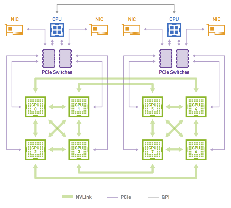
NCCL & Rail Optimization
NCCL stands for NVIDIA Collective Communication Library. It is a library used in applications that need to do collective, cross-GPU actions. It’s topology-aware and allows an abstracted interface to the set of GPUs being used across a cluster system, such that applications don’t need to understand where a particular GPU resides.
Rail Optimization
In a Rail-Optimized topology, each NIC is connected to a different switch (or spine-leaf network) and is called a rail (often represented by a unique color in architecture diagrams). The rails are also interconnected at an upper tier. Therefore, this topology provides two ways to cross rails: through the Scale Up fabric (preferred) or through the upper tier of the Scale Out topology.
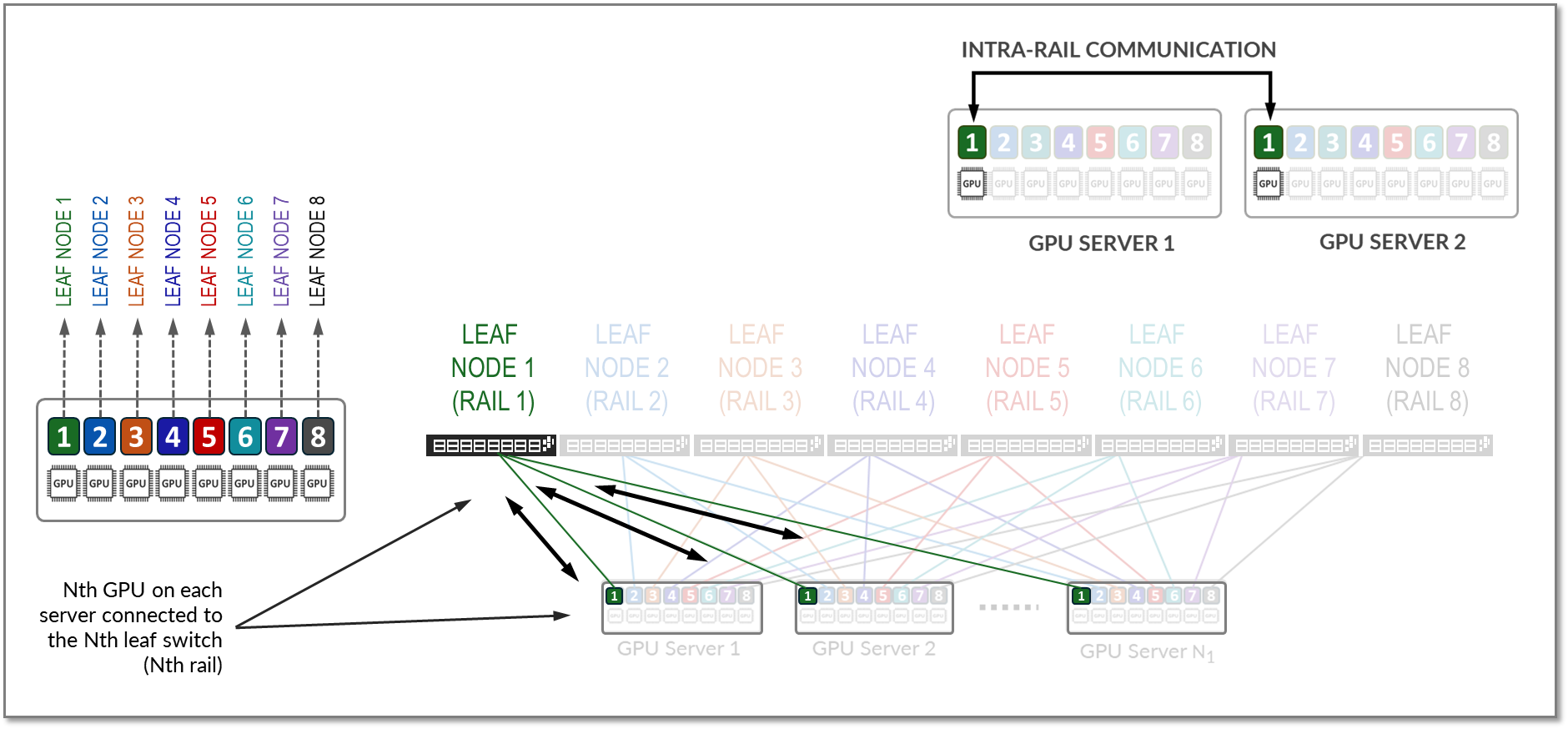
For example, to communicate with GPU 8 on server 2, GPU 4 on server 1 can either:
- Transfer its data into the memory of GPU 8 on server 1. Then GPU 8 on server 1 communicates through NIC 8 on server 1 with GPU 8 on server 2, through NIC 8 on server 2.
- Send its data to NIC 4 on server 1, which can reach through the upper tier to NIC 8 on server 2, coupled with GPU 8 on server 2.
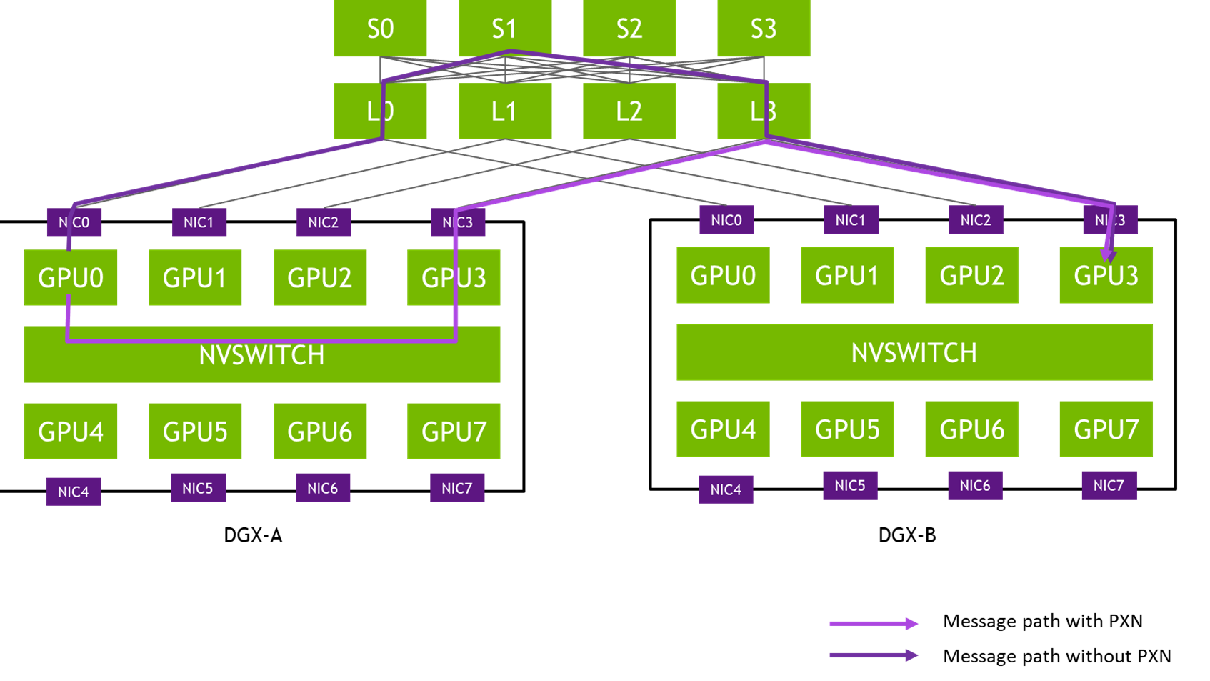
This property allows AI workloads to perform better on a Rail-Optimized topology than on a Pure Rail topology because the current Collective Communication Libraries are not yet fully optimized for the Pure Rail topology. As such, the Rail-Optimized topology is the recommended topology to build a Scale Out fabric.
Network Topologies: Leaf-Spine (CLOS) vs Fat-Tree
Distributed training workloads require predictable, high-bandwidth communication. Different topologies handle this scaling in various ways.
Leaf-Spine (CLOS)
A two-tier architecture where every Leaf switch (connected to servers) is connected to every Spine switch.
- Predictable Latency: Any-to-any communication is always a fixed number of hops.
- East-West Optimization: Optimized for server-to-server traffic rather than client-server (North-South).
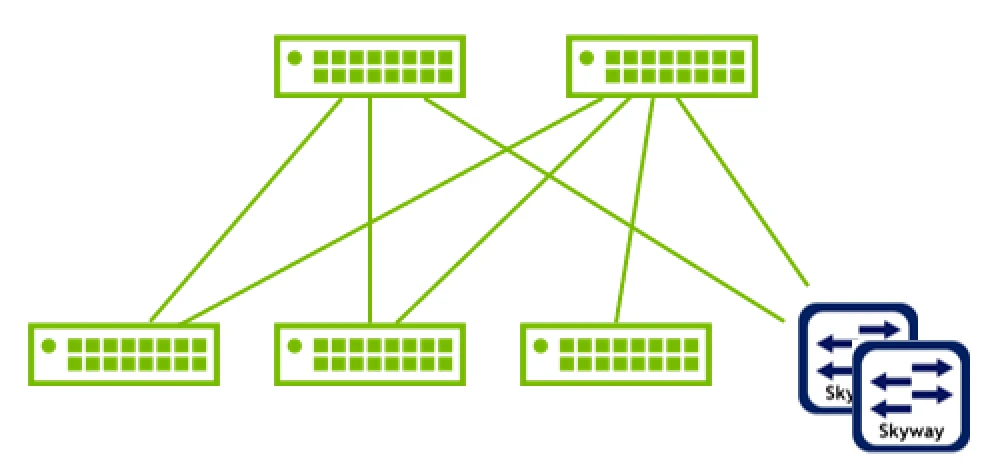
Fat-Tree
A specific, non-blocking implementation of a CLOS network often used in InfiniBand. It is hierarchical but “fat” because the aggregate bandwidth remains constant (or increases) as you move up the tiers toward the root.
- Non-Blocking: Designed so that if all leaves communicate simultaneously, the core can handle the total bandwidth without congestion.
- Scalability: Can scale to three or more stages (Edge, Aggregation, Core) to support thousands of nodes.
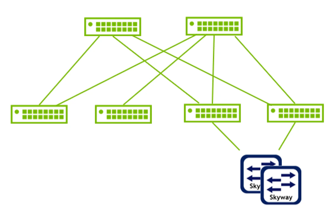
Comparison Table
| Feature | InfiniBand | RoCE v2 | TCP/IP |
|---|---|---|---|
| Transport | Native IB | UDP/IP (Ethernet) | TCP/IP |
| Flow Control | Credit-based | PFC/ECN | Software |
| Latency | Extremely Low | Low | Higher |
Last updated: 2026-03-07
High-Performance Networking
In GPU clusters and HPC (High-Performance Computing), standard TCP/IP networking often becomes a bottleneck due to high CPU overhead, latency, and frequent context switching. Technologies like RDMA, InfiniBand, and RoCE provide the low-latency, high-throughput interconnects required for distributed AI training.
RDMA (Remote Direct Memory Access)
RDMA allows a computer to access memory on another computer directly, bypassing the operating system kernel and the CPU of the remote machine.
graph LR
    subgraph Node A
        AppA[Application] -- "RDMA Write" --> NIC_A[HCA/NIC]
        MemA[Memory]
    end

    subgraph Node B
        AppB[Application]
        MemB[Memory]
        NIC_B[HCA/NIC]
    end

    NIC_A -- "Direct Data Transfer" --> NIC_B
    NIC_B -- "Write to Memory" --> MemB

    style AppA fill:#f9f,stroke:#333
    style AppB fill:#f9f,stroke:#333
    style NIC_A fill:#bbf,stroke:#333
    style NIC_B fill:#bbf,stroke:#333
- Zero-Copy: Data is transferred directly into memory without being copied to intermediate buffers in the OS.
- Kernel Bypass: Applications communicate directly with the network hardware (NIC), avoiding kernel system calls.
- Lower CPU Utilization: The NIC handles the protocol logic, freeing up the CPU for compute tasks.
InfiniBand (IB)
InfiniBand is a lossy-free, credit-based network architecture designed from the ground up for high-performance computing.
- Credit-Based Flow Control: Unlike Ethernet, which drops packets during congestion, IB uses a hardware-level credit system to ensure packets are only sent when the receiving buffer has space.
- Subnet Manager (SM): A centralized control agent (running on a switch or host) that manages routing and network configuration.
- Low Latency: Latency is typically measured in sub-microsecond ranges.
- Speed Generations:
- HDR: 200 Gbps
- NDR: 400 Gbps (NDR200) or 800 Gbps
RoCE (RDMA over Converged Ethernet)
RoCE brings RDMA capabilities to standard Ethernet networks.
RoCE v1
- Layer 2 Protocol: Encapsulated in the Ethernet link layer.
- Limitation: Not routable beyond a single subnet (L2 only).
RoCE v2
- Layer 3 Protocol: Encapsulated in UDP/IP.
- Routable: Can cross router boundaries, making it more scalable for large data centers.
Lossless Requirement (Convergence)
Standard Ethernet is “lossy” (it drops packets). To support RDMA effectively, Ethernet must be made “lossless” using:
- PFC (Priority Flow Control): Pauses traffic on specific priorities (queues) to prevent buffer overflows.
- ECN (Explicit Congestion Notification): Informs the sender to slow down before buffers are full.
Comparison Table
| Feature | InfiniBand | RoCE v2 | TCP/IP |
|---|---|---|---|
| Transport | Native IB | UDP/IP (Ethernet) | TCP/IP |
| Flow Control | Credit-based (Hardware) | PFC/ECN (Network configuration) | Congestion Avoidance (Software) |
| Latency | Extremely Low (< 1µs) | Low (~2-5µs) | Higher (> 10-20µs) |
| CPU Overhead | Minimal (RDMA) | Low (RDMA) | High (Protocol stack) |
| Deployment | Specialized Infrastructure | Converged (Standard Switches) | Ubiquitous |
Last updated: 2026-03-02
GPU Storage & Parallel Filesystems
High-performance AI training requires storage that can keep up with thousands of concurrent GPU requests.
Parallel Filesystems
Distribute data and metadata across multiple servers to enable linear scaling.
- Lustre: The veteran HPC filesystem. Uses Object Storage Servers (OSS) and Metadata Servers (MDS). Powerful but complex.
- WEKA (WekaFS): Modern, flash-native software-defined storage. Optimized for NVMe and RoCE/IB. Excellent for “small file” AI problems.
GPUDirect Storage (GDS)
Avoids the “CPU Bounce Buffer” by creating a direct DMA path between storage (or network) and GPU memory.
graph LR
    Storage[Parallel Storage] -- "Traditional" --> CPU[CPU/RAM]
    CPU -- "Bounce Buffer" --> GPU[GPU Memory]

    Storage -- "GPUDirect Storage" --> GPU
Benefits
- Reduced end-to-end latency.
- Significant reduction in CPU utilization during I/O.
- Higher overall throughput for I/O-bound training jobs.
Storage Comparison
| Feature | NFS/NAS | Lustre | WEKA |
|---|---|---|---|
| Architecture | Centralized | Distributed | Distributed (SW-Defined) |
| GDS Support | Limited | Yes | Yes (Native) |
| Optimization | General | Bandwidth | NVMe / Small Files |
Last updated: 2026-03-07
Parallel Filesystems for HPC & AI
High-performance AI training and simulation workloads require storage that can keep up with thousands of GPUs. Traditional NAS (NFS/SMB) often becomes a bottleneck due to metadata overhead and serial access patterns.
Why Parallel Filesystems?
Parallel filesystems distribute data and metadata across multiple servers, allowing clients to access data in parallel.
- Striping: Files are broken into chunks (stripes) and spread across multiple storage targets.
- Separation of Data and Metadata: Metadata operations (ls, open, stat) are handled by dedicated Metadata Servers (MDS), while data is served by Object Storage Servers (OSS).
- Scalability: Performance scales linearly by adding more storage or metadata nodes.
Lustre
A veteran in the HPC world, powering many of the world’s largest supercomputers.
- Architecture: Consists of Management Server (MGS), Metadata Servers (MDS), and Object Storage Servers (OSS).
- Open Source: Widely adopted and well-understood in academic and research environments.
- Performance: Capable of TB/s throughput but requires significant expertise to tune and manage.
WEKA (WekaFS)
A modern, software-defined parallel filesystem designed for NVMe and low-latency networking (Infiniband/RoCE).
- Flash-Native: Optimized specifically for NVMe, avoiding the legacy overhead of disk-based filesystems.
- Zero-Copy: Uses DPDK to bypass the kernel, providing local-disk-like performance over the network.
- AI-Focused: Excellent at handling the “small file problem” (millions of small images/tensors) common in deep learning.
GPUDirect Storage (GDS)
A critical technology for modern AI infrastructure that allows a direct DMA (Direct Memory Access) path between GPU memory and storage.
graph LR
    Storage[Parallel Storage] -- "Traditional" --> CPU[CPU/RAM]
    CPU -- "Bounce Buffer" --> GPU[GPU Memory]

    Storage -- "GPUDirect Storage" --> GPU
- Benefit: Bypasses the CPU “bounce buffer,” reducing latency and CPU utilization.
- Requirement: Supported by WEKA, Lustre (via NVIDIA’s client), and others.
| Feature | NFS | Lustre | WEKA |
|---|---|---|---|
| Architecture | Centralized | Distributed | Distributed (Software-Defined) |
| Media | Any | HDD/SSD | Optimized for NVMe |
| Metadata | Serial | Parallel (via MDS) | Distributed & Parallel |
| Complexity | Low | High | Medium |
| GDS Support | Limited | Yes | Yes (Native) |
Last updated: 2026-03-02
Concepts
Virtualization: KubeVirt
Virtualization with KubeVirt
KubeVirt extends Kubernetes by providing Custom Resource Definitions (CRDs) and additional controllers that allow virtual machines (VMs) to run side-by-side with containers in the same cluster. Instead of running a container process directly, KubeVirt launches a standard Pod (the virt-launcher Pod) which encapsulates a libvirt instance and the actual qemu virtualization process.
VM Networking (The TAP Interface)
A key challenge in KubeVirt is connecting the traditional container network provided by a CNI to the virtual machine operating inside the Pod. The CNI provides an interface inside the Pod’s network namespace, but a virtual machine running under libvirt/qemu expects to connect to a virtualization-friendly device, specifically a TAP device (tap0 or vnet0).
KubeVirt bridges this gap using a series of network setup steps executed inside the virt-launcher pod before the VM starts (SetupPodNetwork):
graph TD
    subgraph sg_vm[Virtual Machine]
        eth0_vm["eth0<br/>(Configured by DHCP)"]:::whiteClass
    end

    subgraph sg_pod[Compute Container]
        vnet0["vnet0<br/>(Configured by Libvirt)"]:::tapClass
        br1["br1"]:::bridgeClass
        eth0_pod["eth0<br/>(Configured by CNI)"]:::vethClass

        dhcp(("DHCP")):::tapClass
        virt_launcher["Modified by virt-launcher"]:::tapClass

        virt_launcher --- dhcp
        dhcp --> br1

        vnet0 --- br1
        br1 --- eth0_pod
    end

    subgraph sg_node[Node]
        veth_node["veth#"]:::vethClass
        cni0["cni0<br/>(Configured by CNI)"]:::bridgeClass
    end

    eth0_vm --- vnet0
    eth0_pod --- veth_node
    veth_node --- cni0

    classDef vethClass fill:#fdc87d,stroke:#333,stroke-width:1px,color:#000;
    classDef tapClass fill:#b5e196,stroke:#333,stroke-width:1px,color:#000;
    classDef bridgeClass fill:#8ecae6,stroke:#333,stroke-width:1px,color:#000;
    classDef whiteClass fill:#ffffff,stroke:#333,stroke-width:1px,color:#000;
- Network Discovery: The pre-start hook gathers the IP address, routing table, MAC address, and gateway assigned to the Pod’s
eth0interface by the CNI. - Interface Modification:
- The Pod’s
eth0is brought down, and its assigned IP address is removed. - A layer 2 bridge (e.g.,
br1ork6t-eth0) is created inside the Pod’s network namespace. - The Pod’s
eth0is attached to this new bridge.
- The Pod’s
- TAP Device Connection: A TAP device is created and attached to the same bridge. This TAP interface is injected into
libvirtto act as the backend for the virtual machine’s virtual network card. - IP Re-assignment (Single-Client DHCP): KubeVirt spawns a lightweight DHCP server listening exclusively on the local bridge. When the guest VM boots, it sends a DHCP request over its virtual NIC. The local DHCP server responds by handing the VM the exact IP address, routing configuration, and DNS settings (read from the Pod’s
/etc/resolv.conf) that the CNI originally assigned to the Pod.
As a result, the virtual machine effectively “steals” the Pod’s IP address. Traffic destined for the VM hits the CNI, transverses into the Pod’s eth0, crosses the bridge to the TAP device, and is swallowed by the VM’s guest OS.
Network Binding Plugins
Historically, the strategies used to connect the TAP device and the Pod interface (e.g., Bridge, Masquerade, Passt, Slirp) were hardcoded in KubeVirt core:
- Bridge: Connects the TAP and internal interfaces to the same layer 2 bridge, seamlessly passing L2 traffic.
- Masquerade: Leaves the IP on the Pod interface and uses
iptablesNAT rules to route traffic to the TAP device, effectively hiding the VM behind the Pod IP. - Slirp/Passt: Implement traffic redirection using a user-space network stack, which is useful when kernel privileges (like creating bridges/taps) are restricted.
To improve customizability and address shortcomings like difficult dual-stack IPv6 configurations, KubeVirt abstracted these setups into Network Binding Plugins. Operating via gRPC (similar to Hook Sidecars), these plugins intercept the VM creation process at specific hooks (onDefineDomain and preCloudInitIso). This allows external network components to dynamically manipulate the libvirt XML definition and cloud-init user data, completely customizing how the TAP device behaves and connects without requiring changes to the core KubeVirt codebase.
Concepts
Networking: Fundamentals
Networking Fundamentals
Understanding how data moves across the network is essential for debugging connectivity and performance issues in distributed systems.
TCP vs. UDP
| Feature | TCP (Transmission Control Protocol) | UDP (User Datagram Protocol) |
|---|---|---|
| Connection | Connection-oriented (Handshake) | Connectionless (Fire & Forget) |
| Reliability | Guarantees delivery (Retransmission) | No guarantee (Best effort) |
| Ordering | Guarantees packet order | No guarantee |
| Speed | Slower (Overhead of ACKs) | Faster (Minimal overhead) |
| Examples | HTTP, SSH, SMTP, PostgreSQL | DNS (often), VoIP, Streaming |
The TCP 3-Way Handshake
Before any data is sent, a TCP connection must be established:
- SYN: Client sends a Synchronize packet with a random Sequence Number ($X$).
- SYN-ACK: Server acknowledges with its own Sequence Number ($Y$) and sets ACK to $X+1$.
- ACK: Client acknowledges by setting ACK to $Y+1$.
DNS Record Types
The Domain Name System (DNS) translates hostnames to IP addresses using various record types:
- A: Maps a hostname to an IPv4 address.
- AAAA: Maps a hostname to an IPv6 address (16 bytes).
- CNAME: An alias from one domain name to another (Canonical Name).
- MX: Mail Exchange record (where to send emails).
- PTR: Pointer record for Reverse DNS lookups (IP to hostname).
- TXT: Arbitrary text data (used for SPF, DKIM, DMARC validation).
Common Port Numbers
Ports allow multiple services to share a single IP address. There are 65,535 TCP/UDP ports. Ports < 1024 are privileged.
| Protocol | Port | Description |
|---|---|---|
| DNS | 53 | Name resolution |
| SSH | 22 | Secure shell access |
| HTTP | 80 | Unencrypted web traffic |
| HTTPS | 443 | Encrypted web traffic |
Troubleshooting Tools & Logic
The “Golden Path”
When an app can’t connect, follow this flow:
ping [IP]: Is the host alive? (ICMP)dig [hostname]: Is DNS resolving correctly?curl -v [URL]: Is the application level responding?
Traceroute
Uses the TTL (Time To Live) field in IP packets. Each router decreases TTL by 1. When it hits 0, the router sends an ICMP “Time Exceeded” message back, allowing traceroute to map the path.
Checking Open Ports
ss -tlpn: (Socket Statistics) Modern replacement fornetstat.lsof -i :port: Shows the process using a specific port.
HTTP Response Codes
- 2xx: Success (e.g., 200 OK)
- 3xx: Redirection
- 4xx: Client Error (e.g., 404 Not Found, 403 Forbidden)
- 5xx: Server Error (e.g., 500 Internal Error, 502 Bad Gateway)
Last updated: 2026-03-26
Concepts
Networking: DHCP
DHCP (Dynamic Host Configuration Protocol)
DHCP is a network management protocol used on Internet Protocol (IP) networks for automatically assigning IP addresses and other communication parameters to devices connected to the network using a client–server architecture.
DHCP Phases
The standard IP allocation process follows the DORA sequence (Discover, Offer, Request, Acknowledge):
sequenceDiagram
    participant Client
    participant Server as DHCP Server

    Client->>Server: DISCOVER: Discover all DHCP servers on subnet
    Server-->>Client: OFFER: Server receives ethernet broadcast and offers IP address
    Client->>Server: REQUEST: Client sends REQUEST broadcast on subnet using offered IP.
    Server-->>Client: ACK: Server responds with unicast and ACKs request.
Explaining the Phases
While DORA covers the standard successful assignment, the full DHCP protocol includes other critical phases to handle conflict and lifecycle management:
- DISCOVERY: The client broadcasts a DHCPDISCOVER message on the local physical subnet to find available DHCP servers. Since the client doesn’t have an IP address yet and doesn’t know the server’s IP, it uses the broadcast address
255.255.255.255. - DECLINE: During the DORA process, if the client determines that the offered IP address is already in use on the network (e.g., via an ARP probe), it sends a
DHCPDECLINEmessage to the server. The process then starts over again with a new DISCOVERY phase. - RELEASE: When the client gracefully disconnects or no longer needs the network address (e.g., upon shutdown), it sends a
DHCPRELEASEmessage to the server, allowing the IP address to be returned to the pool for reallocation to another device.
Concepts
Networking: DNS
DNS (Domain Name System)
The Domain Name System (DNS) translates human-readable domain names (like example.com) to machine-readable IP addresses.
Complete DNS Lookup and Webpage Query
The full resolution and connection process involves multiple layers of caching and a hierarchical search across global DNS infrastructure.
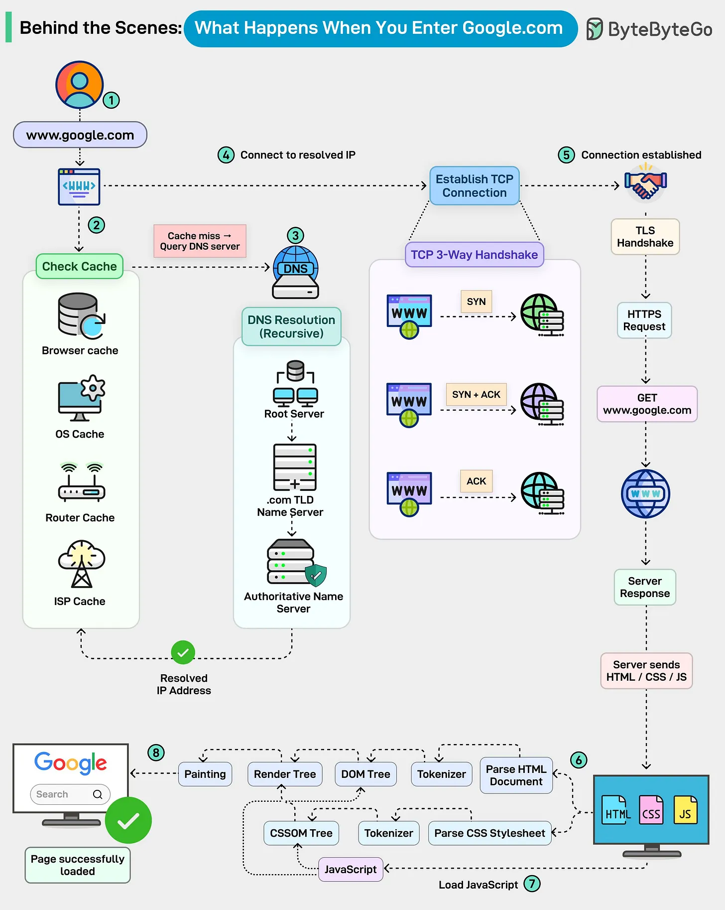
The 4 Layers of DNS Caching
Before reaching out to the network, the system checks several cache layers for a quick hit:
- Browser Cache: The browser maintains its own temporary database of DNS records for recently visited sites.
- OS Cache: If not in the browser, the OS (via a “stub resolver”) checks its own local cache (
hostsfile or internal DNS cache). - Router Cache: Many home/office routers maintain their own DNS cache to speed up requests for all devices on the network.
- ISP DNS Cache: If all else fails locally, the recursive resolver at your ISP (Internet Service Provider) is queried, which often has a large cache of popular domains.
Recursive vs. Iterative Queries
If the IP is not cached, the Recursive DNS Resolution begins:
- Recursive Query: The client asks the DNS Resolver (usually provided by the ISP or a public provider like 8.8.8.8) for the final answer. The resolver takes full responsibility for the search.
- Iterative Queries: The Resolver performs the “heavy lifting” by querying the hierarchy:
- Root Servers: Directed to the correct TLD Server (e.g.,
.com). - TLD Name Servers: Directed to the Authoritative Name Server for the specific domain (e.g.,
google.com). - Authoritative Name Servers: Provides the final A Record (IP Address) back to the resolver.
- Root Servers: Directed to the correct TLD Server (e.g.,
Connection & Rendering
Once the IP is returned to the browser:
- TCP 3-Way Handshake: SYN → SYN/ACK → ACK.
- TLS Handshake: Secure encryption is established.
- HTTP Request: The browser sends the GET request; the server responds with resources (HTML, CSS, JS).
- Rendering: The browser parses the DOM/CSSOM, constructs the Render Tree, and paints the page.
Concepts
System Design: Distributed Systems
Consistent Hashing (The Scalability Backbone)
In a distributed system, we often need to map keys to servers (e.g., in a DHT or for Load Balancing).
The Rehashing Problem
Traditional hashing uses $index = hash(key) \pmod n$. If $n$ (number of servers) changes, almost all keys are remapped, leading to a cache miss storm.
How Consistent Hashing Works
Consistent Hashing maps both servers and keys onto a circular hash space (a Hash Ring).

- Placement: Both keys and servers are hashed to positions on the ring.
- Assignment: A key is assigned to the first server it encounters moving clockwise.
- Minimal Disruption: When a node is added/removed, only $K/N$ keys need remapping on average (where $K$ is the number of keys and $N$ is the number of slots). This is the “minimal disruption” property.
Virtual Nodes (Smoothing & Hotspots)
Physical nodes can be unevenly distributed, leading to the Hotspot Key Problem. Virtual Nodes map multiple points on the ring to a single physical server.
- Uniformity: Increasing virtual nodes reduces the standard deviation of load distribution.
- Balance: If one server is more powerful, it can be assigned more virtual nodes.
CAP Theorem: The Distributed Trade-off
The CAP theorem states that a distributed data store can only provide two of the following three guarantees:
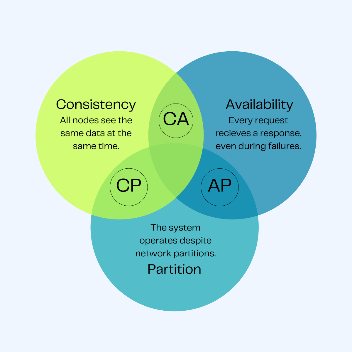
- Consistency (C): Every read receives the most recent write or an error.
- Availability (A): Every request receives a (non-error) response, without the guarantee that it contains the most recent write.
- Partition Tolerance (P): The system continues to operate despite an arbitrary number of messages being dropped (or delayed) by the network between nodes.
The C vs A Choice
Since network partitions (P) are inevitable in distributed systems, the real choice is between Consistency and Availability:
- CP (Consistency/Partition Tolerance): If a partition occurs, the system stops accepting writes to ensure consistency. (e.g., etcd, ZooKeeper).
- AP (Availability/Partition Tolerance): The system continues to accept writes/reads, potentially returning stale data. (e.g., Cassandra, DynamoDB).
Bloom Filters (Memory-Efficient Check)
A Bloom Filter is a probabilistic data structure used to check if an element is a member of a set.

- Result 1: “Definitely not in the set” (100% certain).
- Result 2: “Possibly in the set” (False positives are possible).
How it works
- Initialize a bit-array of $m$ bits to all 0s.
- To add an element: Run it through $k$ different hash functions and set the corresponding bits in the array to 1.
- To check: Run the query through the same $k$ hash functions. If any bit is 0, the element is definitely not there.
[!TIP] Real-world Use: Cassandra and Bigtable use Bloom Filters to avoid expensive disk lookups for keys that don’t exist in an SSTable.
Service Discovery: etcd vs Consul vs ZooKeeper
| Tool | Consensus | Discovery Mechanism | Primary Use Case |
|---|---|---|---|
| etcd | Raft | HTTP/gRPC (Watch) | Kubernetes state, Configuration. |
| Consul | Raft / Gossip | DNS / HTTP / gRPC | Service Mesh, Health checking. |
| ZooKeeper | ZAB (Paxos-like) | Client Library (Watches) | Hadoop, Kafka, complex coordination. |
Gossip Protocols (Discovery & Membership)
Gossip protocols are peer-to-peer protocols inspired by the way rumors spread in a social network. They are highly scalable and resilient, used for failure detection and metadata dissemination.

SWIM (Scalable Weakly-consistent Infection-style Process Group Membership Protocol)
SWIM separates the failure detection from the membership dissemination.
Mechanisms:
- Failure Detection: A node
Arandomly selects nodeBand pings it. If no response,Aaskskother nodes to pingB(Indirect Ping). - Dissemination: Membership changes (joins, leaves, failures) are piggybacked on the ping/ack messages.
| Feature | Description |
|---|---|
| Scalability | $O(1)$ load per node, regardless of cluster size. |
| Resilience | No single point of failure; works even with high packet loss. |
| Latency | $O(\log N)$ to propagate information to all nodes. |
[!TIP] Use Case: HashiCorp Consul uses SWIM (via the
memberlistlibrary) for cluster membership and failure detection.
Consensus: The Raft Algorithm
Consensus is the process of getting a group of nodes to agree on a single value or a sequence of operations (the log). Raft is a leader-based consensus algorithm designed for clarity.

[!TIP] Learning Resource: A fantastic visual guide to Raft can be found at The Secret Lives of Data, which explains the algorithm through interactive animations.
How Raft Works: High-Level Concepts
1. Node States
In Raft, a node can be in one of three states: Follower, Candidate, or Leader.
2. Leader Election
If a Follower does not hear from a Leader for an Election Timeout, it becomes a Candidate and asks others for votes. If it receives a majority, it becomes the Leader.
3. Log Replication
The Leader handles all client writes. It appends the change to its log and broadcasts it to followers. Once a majority acknowledge, the change is committed.
Safety & Commit Rules
- Leader Completeness: A leader must have all committed entries from previous terms. If a candidate’s log is less up-to-date than a follower’s, the follower will reject the vote.
- Election Safety: At most one leader can be elected in a given term.
Comparison: Raft vs Paxos
| Feature | Paxos | Raft | | :— | :— | :— | | Philosophy | Based on “Proposers/Acceptors” (Peer-to-peer). | Based on “Leader/Follower” (Centralized). | | Complexity | Extremely difficult to understand and implement. | Designed to be “understandable”. | | Frameworks | Google’s Chubby, Zookeeper (ZAB). | etcd, Consul, CockroachDB. |
Consistency Models
Consistency defines the order in which operations appear to happen to the users of a system.
The Spectrum of Consistency
- Strict/Strong Consistency: Every read returns the most recent write. (Linearizability).
- Sequential Consistency: All processes see the same order of operations, but not necessarily “real-time” latest.
- Causal Consistency: Operations that are causally related are seen in the same order.
- Eventual Consistency: If no new updates are made, all reads will eventually return the same value.
Beyond CAP: The PACELC Theorem
CAP is too simplistic for modern systems. PACELC expands it by considering what happens when there is no partition:
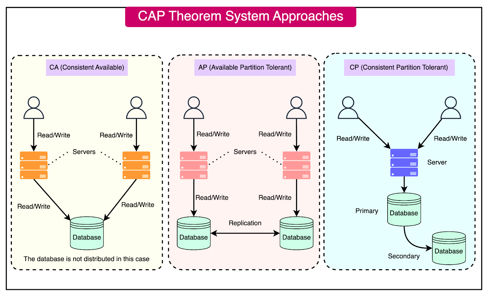
- Partition: If there is a partition (P), how do you choose between Availability (A) and Consistency (C)?
- Else: Else (operating normally), how do you choose between Latency (L) and Consistency (C)?
| System | Partition Behavior | Normal Behavior | Example |
|---|---|---|---|
| DynamoDB | Available | Latency | PA/EL |
| Cassandra | Available | Latency | PA/EL |
| MongoDB | Available | Consistency | PA/EC |
| Fully ACID | Consistent | Consistency | PC/EC |
Real-World Interview Scenario: Designing etcd
How does etcd handle a network partition between the leader and the majority of followers?
- The Leader (isolated) cannot reach a quorum, so it cannot commit new entries.
- The majority side elects a new leader (higher term).
- When the partition heals, the old leader sees the higher term and steps down to Follower.
- The old leader’s uncommitted entries are overwritten by the new leader’s log.
Concepts
System Design: Networking
Load Balancing Architecture: L4 vs L7
Load balancing is the process of distributing network traffic across multiple servers. To design a scalable system, we must choose the right layer for traffic management.
Layer 4 Load Balancing (Transport Layer)
Layer 4 load balancing operates at the Transport Layer (TCP/UDP). It makes routing decisions based on IP addresses and port numbers without inspecting the actual application data.
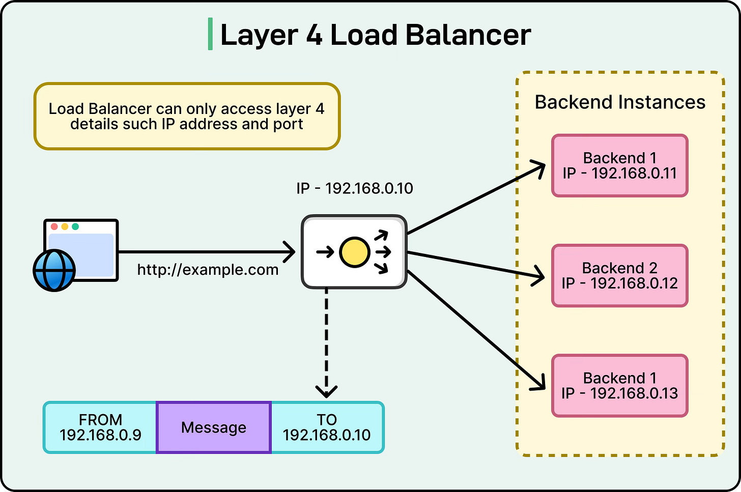
- Mechanism: Uses Network Address Translation (NAT) or Direct Server Return (DSR).
- Pros: Extremely fast, low CPU overhead, handles high-throughput traffic easily.
- Cons: No visibility into HTTP headers, cookies, or URLs; cannot perform content-based routing.
Layer 7 Load Balancing (Application Layer)
Layer 7 load balancing operates at the Application Layer (HTTP/HTTPS/gRPC). It terminates the client’s network connection and inspects the payload to make intelligent routing decisions.
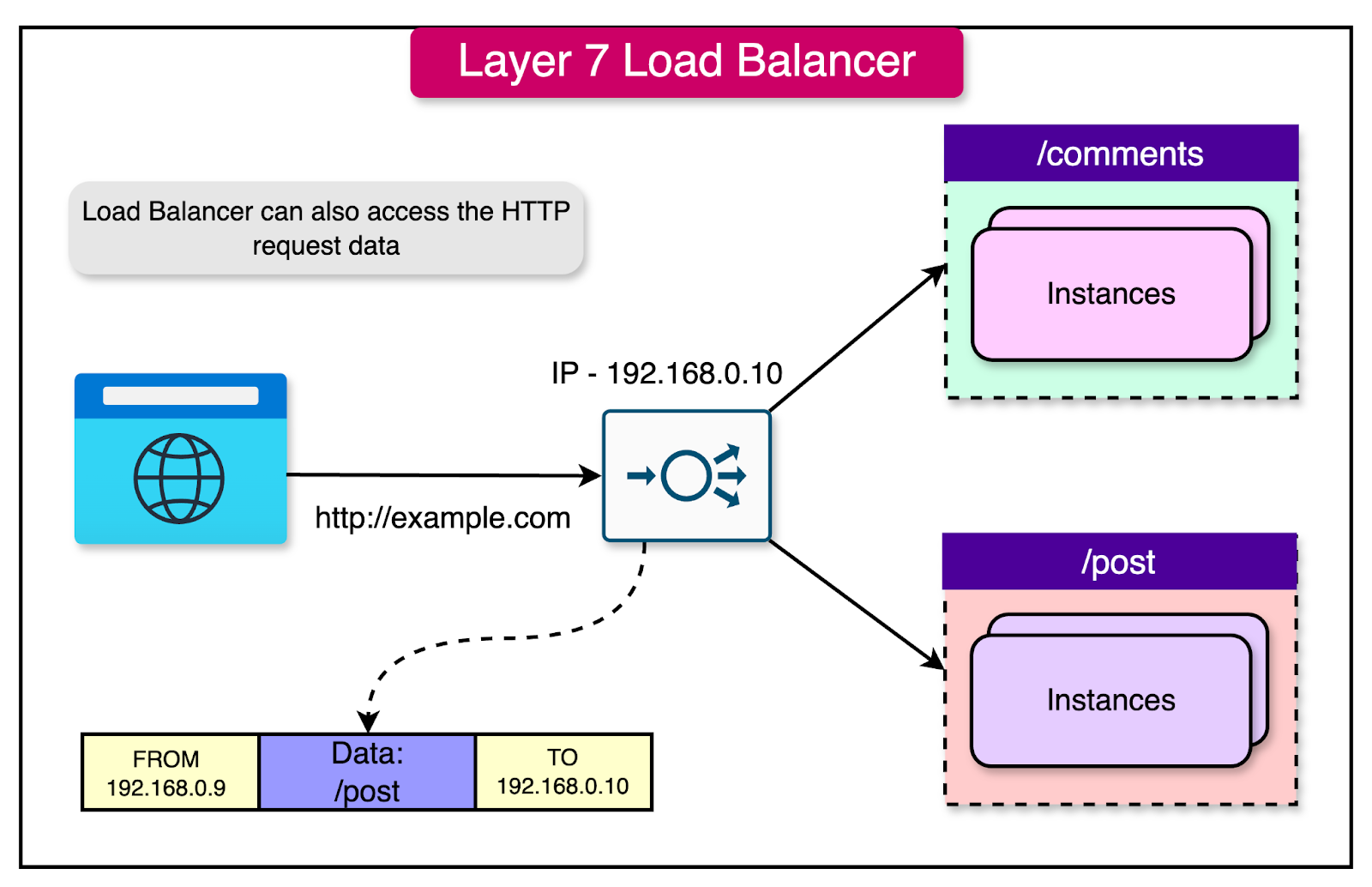
- Mechanism: Acts as a full proxy. Terminates SSL/TLS, inspects URLs, headers, and cookies.
- Pros: Intelligent routing (path-based, cookie-based), SSL Offloading, Caching, WAF integration.
- Cons: More CPU intensive, higher latency due to connection termination and packet inspection.
Technical Comparison: L4 vs L7
| Feature | L4 (Transport) | L7 (Application) |
|---|---|---|
| Criteria | IP, TCP/UDP Port | URL, Cookies, Headers |
| Logic | Simple, Fast | Complex, Intelligent |
| Performance | Low Latency | Higher Latency |
| Security | Minimal | SSL Termination, WAF |
| Examples | AWS NLB, F5 | AWS ALB, NGINX, Envoy |
Communication Protocols: gRPC vs WebSockets
gRPC (Google Remote Procedure Call)
Modern, high-performance RPC framework that uses HTTP/2 as the transport.
- Mechanism: Uses Protocol Buffers (binary format) for serialization.
- Streaming: Supports client-side, server-side, and bidirectional streaming.
- Pros: Low latency, lightweight payloads, strongly typed (IDL), multiplexing.
- Cons: Requires HTTP/2 support, less “browser-friendly” without a proxy (grpc-web).
WebSockets
Bidirectional, persistent connection between client and server over a single TCP socket.
- Mechanism: Starts as an HTTP request with an
Upgradeheader. Once established, it’s a raw TCP stream. - Pros: Real-time communication, low overhead once connected.
- Cons: Persistent connections consume server resources, requires keeping state (Sticky sessions).
| Feature | gRPC | WebSockets |
|---|---|---|
| Transport | HTTP/2 | TCP (via HTTP Upgrade) |
| Payload | Binary (Protobuf) | Text / Binary (Raw) |
| Lifecycle | Request/Response or Streaming | Persistent Connection |
| Best used for | Microservices, High-perf APIs | Chat, Real-time dashboards |
Polling Mechanisms: Real-time Data Retrieval
How does a client stay updated with server-side changes?
- Short Polling: Client sends requests at regular intervals (e.g., every 5s).
- Cons: High overhead, wasted resources if no data changed.
- Long Polling: Client sends a request, server holds it open until data is available or a timeout occurs.
- Pros: Better than short polling, more “real-time”.
- Cons: Still uses one connection per client.
- Server-Sent Events (SSE): One-way persistent stream from server to client over HTTP.
- Pros: Unidirectional, handles reconnection automatically.
- WebSockets: The “gold standard” for bidirectional real-time communication.
Reverse Proxies & API Gateways
Reverse Proxy vs Forward Proxy
- Forward Proxy: Acts on behalf of the client to hide its identity (e.g., corporate proxy).
- Reverse Proxy: Acts on behalf of the server to provide security, load balancing, and performance (e.g., NGINX).
API Gateway Patterns
An API Gateway is a specialized reverse proxy that handles cross-cutting concerns:
- Authentication/Authorization: Validating JWTs at the edge.
- Rate Limiting: Protecting downstream services.
- Request Transformation: Converting XML to JSON or gRPC to HTTP.
- Observation: Centralized logging and tracing.
Service Discovery
How do services find each other in a dynamic environment?
Client-Side Discovery
- Client queries a Service Registry (e.g., Netflix Eureka).
- Registry returns a list of healthy instances.
- Client chooses an instance using its own load balancing algorithm.
Server-Side Discovery
- Client makes a request to a Load Balancer (e.g., AWS ALB).
- Load Balancer queries the Service Registry (or has a pre-defined target group).
- Load Balancer routes-forward to a healthy instance.
The Sidecar Pattern (Service Mesh)
In modern microservices (Kubernetes), networking logic is often offloaded to a Sidecar Proxy (e.g., Envoy).
graph LR
    subgraph "Pod A"
        AppA[App Container] <--> SidecarA[Envoy Sidecar]
    end
    subgraph "Pod B"
        AppB[App Container] <--> SidecarB[Envoy Sidecar]
    end
    SidecarA -- "mTLS / Tracing / Retries" --> SidecarB
[!IMPORTANT] Interview Question: Why use a Service Mesh like Istio over a central API Gateway?
- Service Mesh handles East-West traffic (service-to-service).
API Gateway handles North-South traffic (external-to-service).
Behind the Scenes: What Happens When You Enter a URL?
This is a classic system design interview question that tests your understanding of the entire web stack, from DNS resolution to browser rendering.
1. DNS Resolution (The “Address Book” Lookup)
The browser first needs the IP address of the server. It checks multiple cache layers: Browser → OS → Router → ISP. If not found, a Recursive DNS Resolution kicks off, querying Root servers, TLD servers (.com), and finally the Authoritative server for the domain.
2. Connection Establishment (The Handshake)
Once the IP is known, the browser establishes a connection:
- TCP 3-Way Handshake: Ensures a reliable connection is established between client and server.
- TLS Handshake: Wraps the connection in encryption for security (HTTPS).
3. HTTP Request & Response
The browser sends an HTTP GET request for the resource. The server processes this (often through load balancers and reverse proxies) and streams back the HTML, CSS, and JavaScript.
4. Browser Rendering (The Painting)
The browser engine takes over to display the page:
- Parsing: Converts HTML to the DOM tree and CSS to the CSSOM tree.
- Render Tree: Combines DOM and CSSOM to determine what’s visible.
- Layout: Calculates the exact position and size of each element.
- Painting: Fills in pixels on the screen.
[!TIP] Performance Optimization: Techniques like DNS Prefetching, TCP Fast Open, and CDN Caching are used to minimize the latency of these steps, making the page feel “instant.”
Concepts
System Design: Storage & Databases
Storage Engines: LSM-Tees vs B-Trees
A storage engine is the low-level component of a database that handles how data is stored on disk and retrieved.
B-Trees (Read-Optimized)
Data is organized into fixed-size pages (usually 4KB). Pages are arranged in a tree structure.
- Mechanism: In-place updates. Modifying a record involves overwriting the page on disk.
- Pros: Fast reads ($O(\log N)$), predictable performance.
- Cons: Slower writes due to “random write” overhead and page fragmentation.
- Example: PostgreSQL, MySQL (InnoDB), Oracle.
LSM-Trees (Write-Optimized)
Data is first written to an in-memory MemTable (sorted) and a Write-Ahead Log (WAL). When the MemTable is full, it’s flushed to disk as an immutable SSTable.
- Mechanism: Append-only. Updates are new versions; deletes are “tombstones”. A background process (Compaction) merges SSTables.
- Pros: Extremely fast sequential writes, high throughput.
- Cons: High “Read Amplification” (must check multiple SSTables) and “Write Amplification” (during compaction).
- Example: Cassandra, RocksDB, LevelDB, Bigtable.
| Feature | B-Trees | LSM-Trees |
|---|---|---|
| Write Speed | Slower (Random I/O) | Faster (Sequential I/O) |
| Read Speed | Faster (Predictable) | Slower (Read Amplification) |
| Storage Layout | Mutable Pages | Immutable Segments |
| Space Overhead | Lower | Higher (due to Compaction) |
Write-Ahead Log (WAL)
The WAL is an append-only log on disk that records every modification before it is applied to the main data structures.
Why is it used?
- Atomicity: Ensures that either all parts of a transaction are applied or none.
- Durability (Recovery): If the database crashes, the system can replay the WAL to reconstruct the state of the in-memory data that hadn’t been flushed to disk yet.
Scaling: Sharding vs Partitioning
Sharding (Horizontal Partitioning)
Splitting a large dataset into multiple smaller databases (Shards) across different servers.
- Key-based Sharding: User ID % Number of Shards.
- Range-based Sharding: Users A-M on Shard 1, N-Z on Shard 2.
- Directory-based Sharding: A discovery service maps keys to shard locations.
Challenges
- Hotspots: One shard getting too much traffic (e.g., celebrity user).
- Joins: Performing joins across shards is extremely expensive.
- Rebalancing: Moving data when adding a new shard.
Replication Strategies
1. Single-Leader
One leader handles all writes. Multiple followers replicate from the leader.
- Sync Replication: Leader waits for follower ACK. (Risk: High latency).
- Async Replication: Leader returns success immediately. (Risk: Data loss if leader fails).
2. Multi-Leader
Multiple nodes handle writes (often across different regions).
- Pros: High availability, low latency for global users.
- Cons: Conflict resolution (Last Write Wins, Causal Ordering).
3. Leaderless (Quorum-based)
Clients send writes to all nodes. A write is successful if it reaches a Quorum.
- $W + R > N$: Ensures that the set of nodes that acknowledged a write and the set of nodes that replied to a read must overlap, ensuring a consistent read.
- Example: Amazon Dynamo, Cassandra.
[!IMPORTANT] Interview Scenario: How do you handle a “Hot Partition” in a sharded database?
- Re-sharding: Use a better shard key (e.g., compound key).
- Hashing: Use a consistent hashing algorithm to distribute load evenly.
- Secondary Indexes: Shard the index differently than the data.
Concepts
System Design: Scalability & Reliability
Caching Strategies
Caching is the process of storing data in a temporary, high-speed storage layer to serve reads faster.
Cache Writing Policies
| Strategy | Description | Pros | Cons | | — | — | — | — | | Write-Through | Write to cache and DB simultaneously. | Data consistency. | High write latency. | | Write-Around | Write to DB only; cache is filled on next read. | Avoids “polluting” cache with one-time writes. | Cache miss on first read. | | Write-Back | Write to cache; write to DB later (asynchronously). | Extremely fast writes. | Data loss if cache fails. |
Cache Eviction Policies
Wait, what happens when the cache is full?
- LRU (Least Recently Used): Evict the item that hasn’t been accessed for the longest time.
- LFU (Least Frequently Used): Evict the item with the lowest access count.
- FIFO (First-In, First-Out): Evict the oldest item.
Rate Limiting Algorithms
Rate limiting prevents a system from being overwhelmed by too many requests.
1. Token Bucket
A “bucket” holds a fixed number of tokens. Each request consumes a token. Tokens are refilled at a fixed rate.
- Pros: Allows for bursts of traffic.
2. Leaky Bucket
Requests are added to a bucket (queue). They are processed at a constant rate. Excess requests “leak” (are dropped).
- Pros: Smooths out traffic; constant processing rate.
3. Sliding Window Counter
Combines the low memory of Fixed Window with the accuracy of Sliding Window Log.
- Mechanism: Approximates the request count in the sliding window using a weighted average of the current and previous fixed-window counters.
Implementation Patterns: Centralized vs Distributed
- Middleware Rate Limiter: Easy to implement, but difficult to scale across multiple server nodes.
- Redis/Memcached Limiter: Centralized store for counters. All application nodes check the same bucket.
- Problem: Race conditions.
- Solution: Use Lua script or Sorted Sets in Redis to ensure atomicity.
Unique ID Generator: Twitter Snowflake
In a distributed system, we need to generate unique, 64-bit, time-sortable IDs without a single point of failure (like a DB auto-increment).
Snowflake 64-bit ID Layout
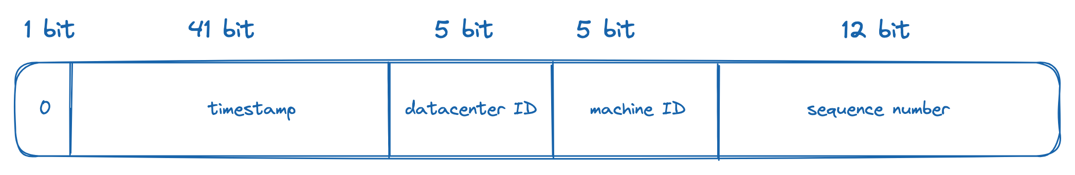
- Sign Bit (1 bit): Always 0 (for positive numbers).
- Timestamp (41 bits): Milliseconds since a custom epoch (e.g., Nov 4, 2010). Lasts ~69 years.
- Datacenter ID (5 bits): Up to 32 datacenters.
- Machine ID (5 bits): Up to 32 machines per datacenter.
- Sequence (12 bits): Incremented for every ID generated on the same machine within the same millisecond. Resets to 0 every millisecond. (Up to 4096 IDs/ms).
Fault Tolerance: The Circuit Breaker Pattern
A circuit breaker prevents an application from repeatedly trying to execute an operation that is likely to fail, allowing it to “fail fast”.
State Machine
stateDiagram-v2
    [*] --> Closed: Normal Operation
    Closed --> Open: Failures > Threshold
    Open --> HalfOpen: Timeout Expired
    HalfOpen --> Closed: Success
    HalfOpen --> Open: Failure
- Closed: Requests are passed through normally.
- Open: Requests are failed immediately (fast fail). No calls are made to the downstream service.
- Half-Open: A limited number of test requests are allowed to check if the service has recovered.
[!IMPORTANT] Interview Scenario: How do you implement an Idempotent API?
- Client-Generated Key: Client sends a unique
Idempotency-Key(e.g., UUID).- Storage: The server stores the key and the response in a database (with TTL).
- Check: On every request, the server checks if the key already exists. If yes, it returns the cached response without re-processing.
Concepts
System Design: Case Studies
Case Study 1: URL Shortener (TinyURL)
Problem: Create a short alias for a long URL (e.g., bit.ly/3xyz).
Core Design
- Hashing Approach: Hash the long URL (MD5/SHA) and take the first 7 characters.
- Problem: Hash collisions.
- Base 62 Conversion: Use a unique 64-bit ID (from a Snowflake generator) and convert it to Base 62 (0-9, a-z, A-Z).
- Example: ID
20,092,156,749,384becomeszn7n9Xj.
- Example: ID
High-Level Architecture
graph LR
    Client -->|POST /shorten| LB[Load Balancer]
    LB --> API[Shortener API]
    API --> ID[ID Generator]
    API --> DB[(SQL/KV Store)]
    Client -->|GET /zn7n9Xj| LB
    LB --> API
    API --> Cache[(Redis)]
    Cache --> Client
Case Study 2: Notification System
Problem: Send real-time notifications to millions of users across different platforms (iOS, Android, Email).
Key Components
- Service Workers: Asynchronous workers that pick up notification tasks from a message queue.
- Third-Party providers: APNS (Apple), FCM (Firebase/Android), Twilio (SMS), SendGrid (Email).
- Aggregation: Batching multiple notifications (e.g., “10 people liked your photo”) to avoid spamming.
Case Study 3: News Feed System
Problem: Scaling a feed like Facebook or Twitter.
Two-Step Flow
- Feed Publishing: When a user posts, the data is stored and pushed to friends’ feeds.
- Fanout-on-Write (Push): Update friends’ feed caches immediately. (Good for fast retrieval, bad for “Celebrity” users with millions of followers).
- Fanout-on-Read (Pull): Build the feed only when the user requests it. (Good for celebrities, bad for latency).
- Feed Retrieval: Fetch consolidated posts from the CDN/Cache.
Case Study 4: Chat System (WhatsApp/Slack)
Problem: Low-latency, bidirectional communication and online presence.
Protocols & Storage
- Protocols: WebSockets for messages (bidirectional), HTTP for login/profile management.
- Presence: A dedicated “Presence Service” maintains user states (online/offline) using a Heartbeat mechanism.
- Storage: NoSQL Key-Value (e.g., Cassandra) is preferred for message history due to high write throughput and easy horizontal scaling.
graph TD
    A[User A] <--> S1[Chat Server 1]
    B[User B] <--> S2[Chat Server 2]
    S1 --> MQ[Message Queue]
    MQ --> S2
    S1 --> Pres[Presence Service]
    Pres --> Redis[(Redis)]
[!TIP] Scaling Presence: During a network partition, use a “Zombie” timeout. If no heartbeat is received for 30s, mark the user offline.